9 Ensemble Forecasts

Good forecasts include measures of uncertainty associated with each forecasted data point. The simulate_ensemble function allows one to make such forecasts. In Calibrating with Observation Error we fitted a model to simulated data with observation error. Here we use this model to illustrate the use of the simulate_ensemble function.

The first thing to do before making a forecast is to extend the end date, so that we are actually forecasting the future.

sir_obs_err_to_forecast = extend_end_date(
  sir_obs_err_calibrated, 
  days_to_extend = 100
)

Next just pass the model that is ready for forecasting to the simulate_ensemble function.

obs_err_forecasts = (simulate_ensemble(
    sir_obs_err_to_forecast, 
    use_progress_bar = FALSE
  )
  %>% filter(var != "S_to_I")
)

The forecasts can be joined back to the observed data to make plots (TODO: fix the naming of the columns of these functions to be more consistent).

obs_err_fits = (obs_err_forecasts
  %>% left_join(
    noisy_data, 
    c("Date" = "date", "var" = "var"), 
    suffix = c("_fitted", "")
  )
  %>% mutate(
    var = factor(
      var, 
      levels = topological_sort(sir_obs_err_to_forecast))
  )
)
(ggplot(obs_err_fits)
  + facet_wrap(~var, scales = 'free', nrow = 2)
  + geom_ribbon(aes(x = Date, ymax = upr, ymin = lwr), alpha = 0.5)
  + geom_point(aes(Date, value), alpha = 0.7)
  + geom_line(aes(Date, value_fitted), colour = "red")
)

## Warning: Removed 833 rows containing missing values (`geom_point()`).

9.1 Time-Varying Ensemble Forecasts

Forecasting often involves exploring what-if-scenarios. For example, what if the transmission rate jumped to high levels in the forecast period due to a policy option under consideration? Such scenario exploration can be done in McMasterPandemic by adding piece-wise time-variation of parameters in the forecasting period using the add_piece_wise function.

sir_tv_to_forcast = (sir_cal_tv
  %>% extend_end_date(days_to_extend = 120)
  %>% add_piece_wise(
    data.frame(
      Date = "2021-01-01",
      Symbol = "beta",
      Value = 0.5,
      Type = "abs"
    )
  )
)

An ensemble forecast can be produced with this scenario model. Here we do just that, while joining back the observed data so that we may plot both the fit and the forecast.

(sir_tv_to_forcast
  %>% simulate_ensemble(use_progress_bar = FALSE)
  %>% filter(var != "S_to_I")
  %>% left_join(
    sir_cal_tv$observed$data,
    c("Date" = "date", "var" = "var"),
    suffix = c("_fitted", "")
  )
  %>% mutate(var = factor(var, topological_sort(sir_cal_tv)))
  %>% ggplot
  + facet_wrap(~var, ncol = 2)
  + geom_line(aes(Date, value))
  + geom_line(aes(Date, value_fitted), colour = 'red')
  + geom_ribbon(aes(x = Date, ymax = upr, ymin = lwr), alpha = 0.5)
)

## Warning: Removed 121 rows containing missing values (`geom_line()`).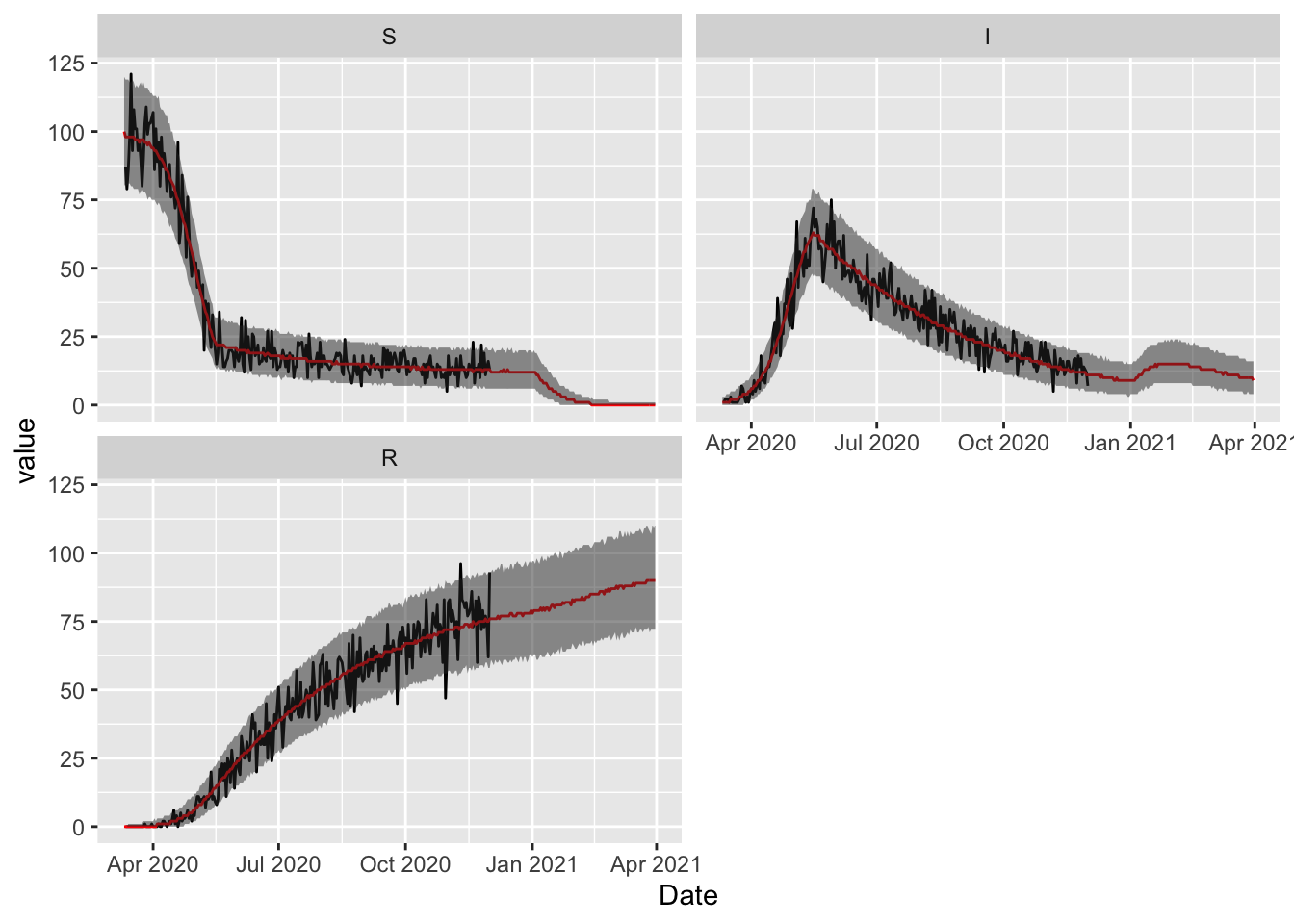

Notice the mini-peak in infected individuals caused by the jump in transmission rate in the forecast period, accompanied by rapid susceptible depletion.