Advanced Calibration

Setup:

library(macpan2)
library(macpan2helpers)
mp2hver <- "0.0.3"
if (packageVersion("macpan2helpers") < mp2hver) {
    stop("please install macpan2helpers version >= ", mp2hver)
}
library(dplyr)
library(tidyr)
library(ggplot2); theme_set(theme_bw())

In addition to these packages, the broom.mixed package and outbreaks package will be used below (if installed).

‘Hello, World’: an easy (??) calibration exercise

We’ll do the first thing you should always do when trying out a new fitting procedure: simulate clean, nice data from the model and see if you can recover something close to the true parameters.

Step 0: set up simulator and generate ‘data’

We will be using several different versions of the SIR model, all of which can be derived from the SIR specification in the model library.

sir_spec = mp_tmb_library("starter_models"
  , "sir"
  , package = "macpan2"
)

From this specification we derive our first version of the model, which we use to generate synthetic data to see if optimization can recover the parameters that we use when simulating.

sir_simulator = mp_simulator(sir_spec
  , time_steps = 100
  , outputs = c("S", "I", "R")
  , default = list(N = 100, beta = 0.2, gamma = 0.1)
)
sir_results = mp_trajectory(sir_simulator)

Add some noise to the prevalence (I) value:

set.seed(101)
sir_prevalence = (sir_results
    |> dplyr::select(-c(row, col))
    |> filter(matrix == "I")
    |> mutate(obs_val = value + rnorm(n(), sd = 1))
)
gg0 <- ggplot(sir_prevalence, aes(time)) +
    geom_point(aes(y = obs_val)) +
    geom_line(aes(y = value))
print(gg0)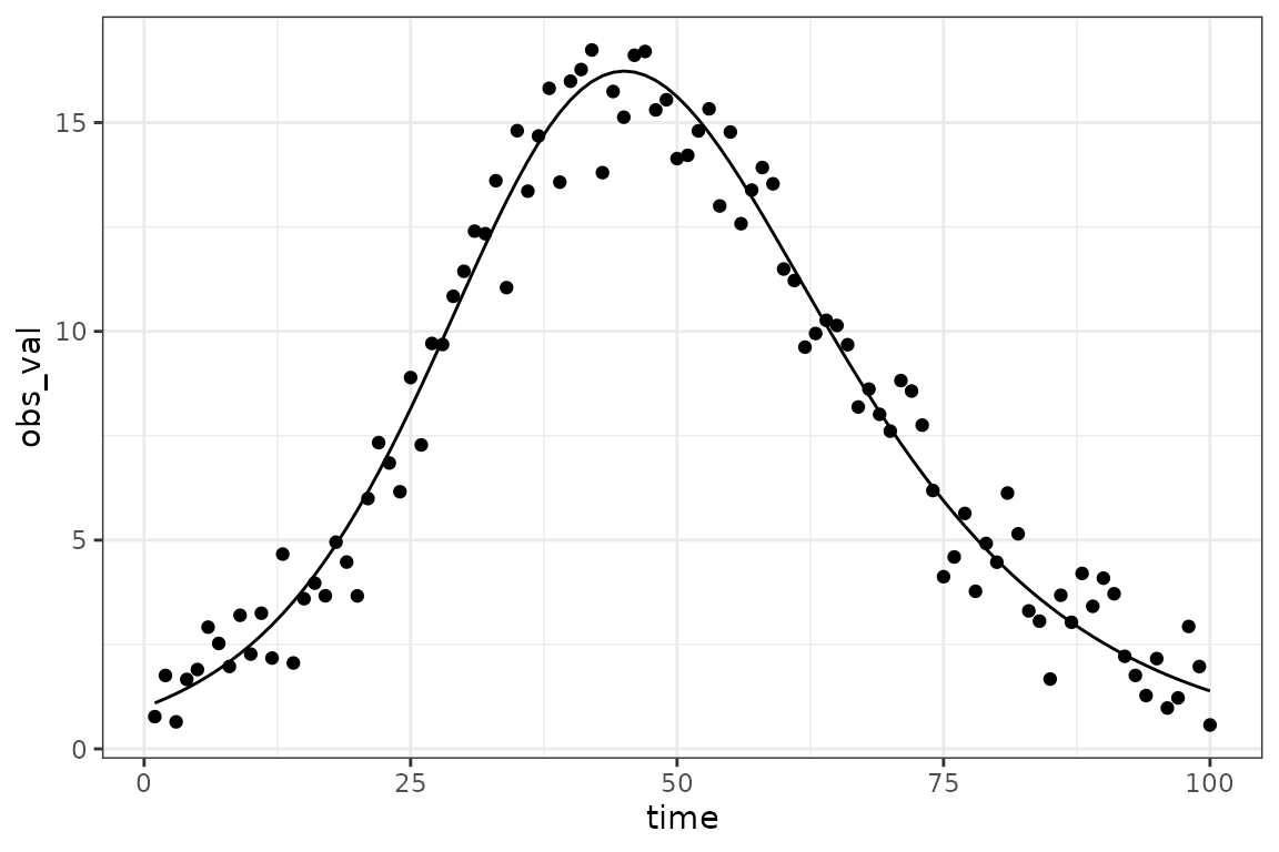

Step 1: add calibration information

Now we’ll use the experimental mk_calibrate() function from macpan2helpers package

macpan2helpers::mk_calibrate(sir_simulator,
   data = data.frame(I_obs = sir_prevalence$obs_val),
   params = list(beta = 1, I_sd = 1),
   transforms = list(beta = "log", I_sd = "log"),
   exprs = list(log_lik ~ dnorm(I_obs, I, I_sd))
)

Unlike typical R functions, this function modifies the sim object in place (!!) FIXME: do not do this in place -- make a clone, which is easy with oor

A sanity check: make sure that the starting values give a reasonable-looking trajectory.

(sir_simulator 
 |> mp_trajectory()
 |> filter(matrix == "I")
 |> ggplot(aes(time, value)) 
 + geom_line()
)

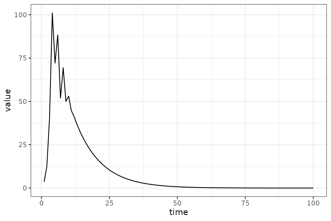
The simulated trajectory is not sensible in this case - the log_beta value is way too large (we set the default to ${\exp(1) \approx}$ 2.72), while we know in this case that the true value is 0.2). Hopefully in a real system we would know enough to get reasonable order-of-magnitude starting values. (If we really knew that $\gamma \approx 0.1$, we would know that a starting value of $\log(\beta)=1$ would correspond to an ${\cal R}_0 \approx 28$, clearly unrealistic for most infectious diseases …

Setting $\log(\beta)=0$ instead gives us a trajectory that is still very unrealistic (the peak of our observed prevalence is only 16.7), but at least it’s smooth. As it turns out this will be good enough, but finding appropriate starting values (based on external information and some trial and error) is often a significant part of a modeling workflow.

(sir_simulator$report(c(0,0)) |>
 filter(matrix == "I") |>
 ggplot(aes(time, value)) + geom_line()
)

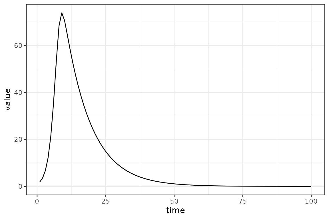
Let’s replace the starting value for log_beta with 0:

sir_simulator$replace$params(
    c(0         , 1         )
  , c("log_beta", "log_I_sd")
)

(In a proper workflow we might prefer to go back upstream to wherever we defined the default values, rather than resetting the value on the fly …)

Step 2: do the fit

fit <- sir_simulator$optimize$nlminb()

Print the results of nlminb - always check the value of the convergence code (if it’s not 0, then something may have gone wrong …)

print(fit)
#> $par
#>      params      params 
#> -1.61413121 -0.07942465 
#> 
#> $objective
#> [1] 133.9514
#> 
#> $convergence
#> [1] 0
#> 
#> $iterations
#> [1] 12
#> 
#> $evaluations
#> function gradient 
#>       18       13 
#> 
#> $message
#> [1] "relative convergence (4)"

Back-transform the parameters:

exp(fit$par)
#>    params    params 
#> 0.1990635 0.9236476

Get more information (this is a little uglier than it should be …)

coefnames <- function(x) {
    x$current$params_frame()$mat
}
drop_trans <- function(x) gsub("(log|logit)_", "", x)

ff <- sir_simulator$ad_fun()
class(ff) <- "TMB"
(broom.mixed::tidy(ff, conf.int = TRUE)
    |> select(-c(type, std.error))
    |> mutate(term = drop_trans(coefnames(sir_simulator)))
    |> mutate(across(where(is.numeric), exp))
    |> as_tibble()
)
#> outer mgc:  1.118671e-09 
#> outer mgc:  63.85069 
#> outer mgc:  63.73186 
#> outer mgc:  0.1998001 
#> outer mgc:  0.2002001 
#> outer mgc:  145.0178
#> # A tibble: 2 × 4
#>   term  estimate conf.low conf.high
#>   <chr>    <dbl>    <dbl>     <dbl>
#> 1 beta     0.199    0.198     0.201
#> 2 I_sd     0.924    0.804     1.06

These correspond to true values of 0.2, 1, so pretty close.

fixme: can we handle back-transformation/parameter naming more nicely? coef(), summary() methods … ??

The best-fit parameters are stored internally, so if we re-run the $report() method we will get information about the predicted best-fit trajectory:

sim_vals <- (sir_simulator
  |> mp_trajectory()
  |> filter(matrix == "I")
)
gg0 + geom_line(data = sim_vals, aes(y= value), colour = "red")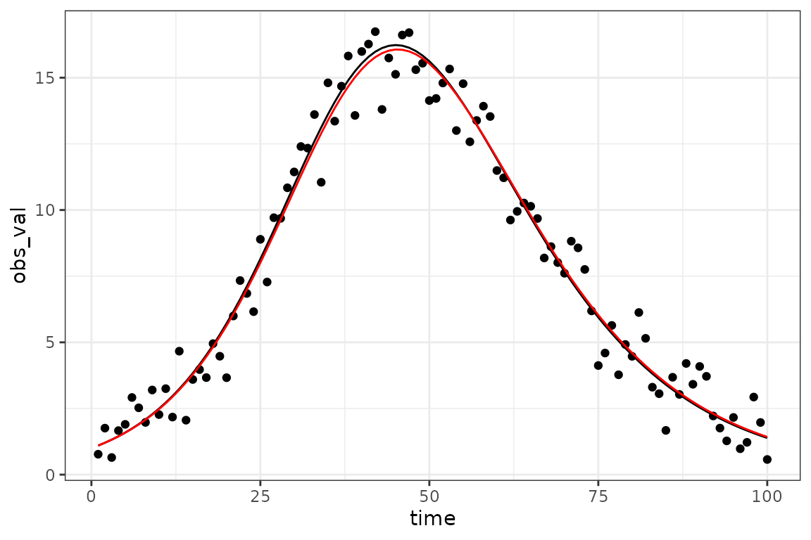

A slightly harder, more realistic example

Here we’ll show off a few alternate choices you could have made. We’ll (1) use real data instead of simulated; (2) fit beta and gamma, (3) use a negative binomial response (which needs a dispersion parameter I_disp instead of a standard deviation …)

library(outbreaks)
sir_simulator = mp_simulator(sir_spec
  , time_steps = 100
  , outputs = c("S", "I", "R")
  , default = list(N = 763, I = 3, beta = 1, gamma = 0.5)
)
macpan2helpers::mk_calibrate(sir_simulator
  , data = data.frame(I_obs = influenza_england_1978_school$in_bed)
  , params = list(beta = 1, gamma = 0.5, I_disp = 1)
  , transforms = list(beta = "log", gamma = "log", I_disp = "log")
  , exprs = list(log_lik ~ dnbinom(I_obs, I, I_disp))
)
sir_simulator$objective(log(c(1, 0.5, 1)))
#> [1] 94.70146

How does this look with our default parameters? (To save typing I’m writing a generic function that runs the model with a specified set of parameters, then plots the results along with the data.)

fixme: some basic plotting functionality in macpan2helpers ?

sim_plot <- function(pars = log(c(1, 0.5, 1))) {
    predvals <- (sir_simulator$report(pars)
        |> filter(matrix == "I")
        |> select(time, I_obs = value)
        |> bind_cols(influenza_england_1978_school)
    )
    ggplot(predvals, aes(time, I_obs)) + geom_line() +
        geom_point(aes(y= in_bed)) +
        labs(x="time", y = "I/'in bed'")
}
sim_plot()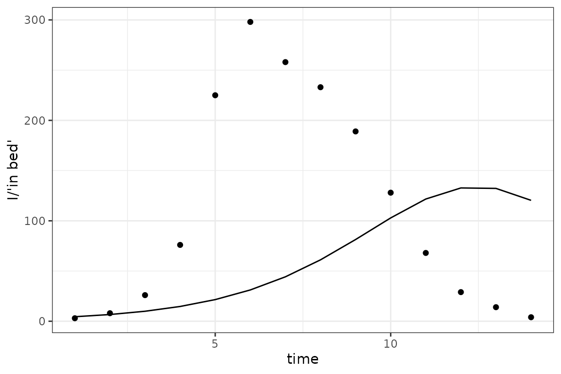

Not great: it helps if we bump up the value of beta (to $\mathcal{R}_0 = 4$):

sim_plot(pars = log(c(2, 0.5, 1)))

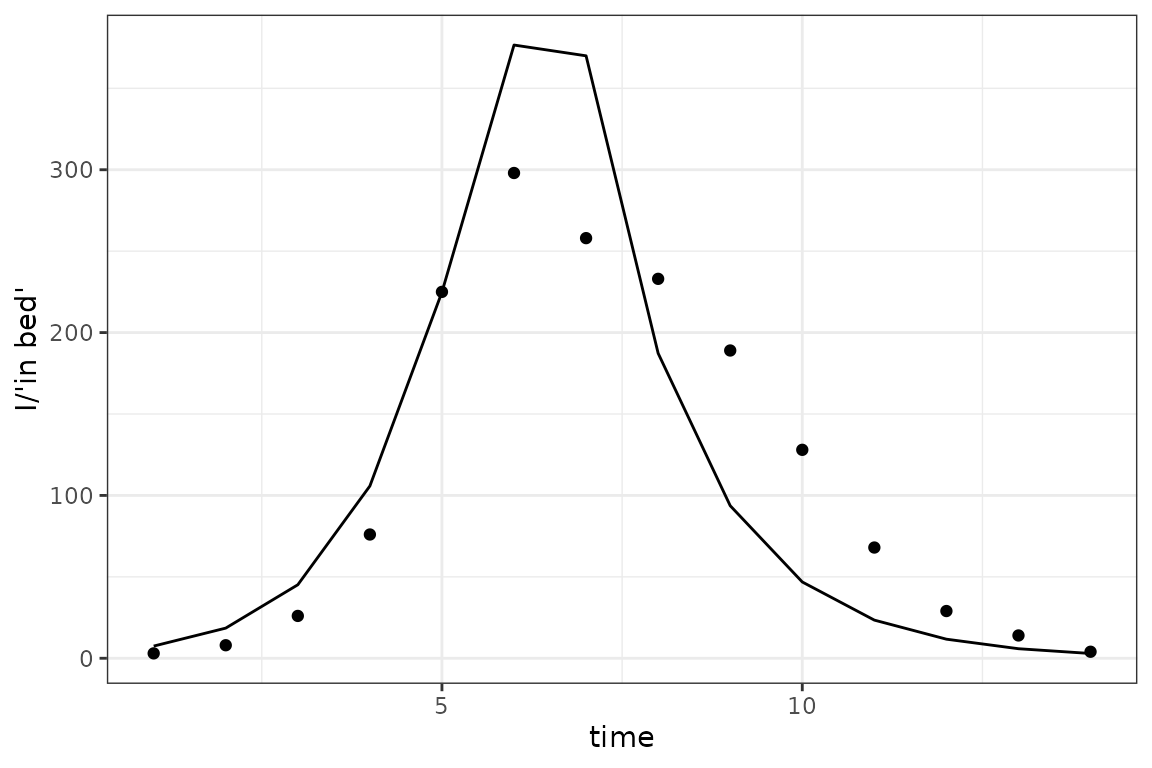
optimize$nlminb() fails (obscurely) for our first set of starting values, but works OK if we increase beta:

fixme: (1) clarify that default parameters need to be transformed (i.e. this does work if we $replace$params(log(c(1, 0.5, 1)), ...)); (2) save loglik values per point so that we can see why the original (untransformed) values (1, 0.5, 1) lead to infinite log-likelihoods, even when we think we’re clamping variables … ?? (The simulated output doesn’t look that crazy …)

sir_simulator$replace$params(log(c(2, 0.5, 1)), c("log_beta", "log_gamma", "log_I_disp"))
fit <- sir_simulator$optimize$nlminb()
#> outer mgc:  38.61651 
#> outer mgc:  16.53627 
#> outer mgc:  6.449698 
#> outer mgc:  48.42602 
#> outer mgc:  33.06605 
#> outer mgc:  2.831973 
#> outer mgc:  0.6015714 
#> outer mgc:  0.009401567 
#> outer mgc:  1.102318e-06

sim_plot(pars = fit$par)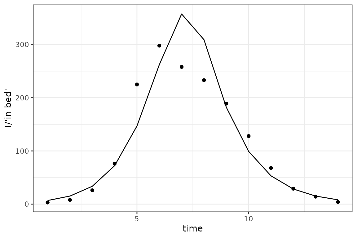

The fit isn’t perfect, but we can think of a number of reasons for that (people are complicated; our model is only tracking the number of current infected children, while the data are numbers of children in bed; we haven’t allowed for an exposed class …).

Computing and plotting confidence and prediction intervals

While this code isn’t horribly complex, hopefully it will all be somewhat more streamlined/automated in the future. Computing confidence or prediction intervals is a fairly big subject; see Bolker (2008) chapter 7 for an introduction to some of the issues.

obs <- data.frame(
    time = seq(nrow(influenza_england_1978_school))
  , value = influenza_england_1978_school$in_bed
)
res = (sir_simulator$report_with_sd()
  |> mutate(
        var = factor(matrix, levels = c("S", "I", "R"))
      , lwr_delta = value - 1.96 * sd
      , upr_delta = value + 1.96 * sd
    )
)
#> outer mgc:  1.102318e-06 
#> outer mgc:  2.135549 
#> outer mgc:  2.137124 
#> outer mgc:  0.5301401 
#> outer mgc:  0.5279329 
#> outer mgc:  0.007252414 
#> outer mgc:  0.007242536
gg_base <- (res
  |> ggplot(aes(x = time, y = value)) 
  + geom_line(aes(colour = var)) 
  + geom_point(data = obs)
)
gg_ci1 <- (gg_base 
  + geom_ribbon(
        aes(ymin = lwr_delta, ymax = upr_delta, fill = var)
      , alpha = 0.3, colour = NA
    )
)
print(gg_ci1)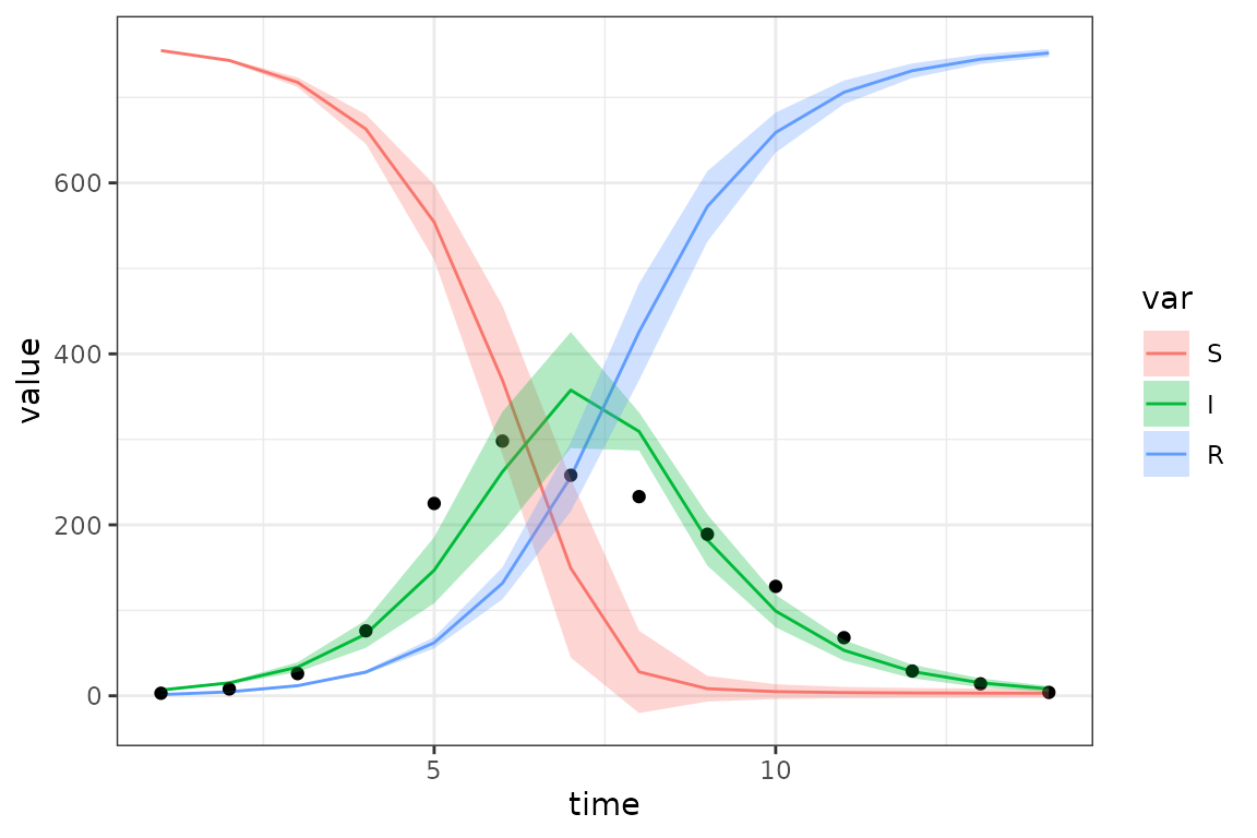

• These intervals are based on the delta method, as such they are approximate (nearly all CIs are approximations, but the delta method assumes both (1) multivariate normality of the sampling distribution and (2) a quadratic approximation to any nonlinearities in the model). You can see that this leads to negative values within the CI range at some points …
• These are confidence intervals, not prediction intervals (so we don’t necessarily expect the points to lie within the envelope); prediction intervals for non-Normal errors are a little bit tricky (maybe something about this in Bolker 2008?), not worth doing right now.

We can also generate intervals based on multivariate normal sampling, which relaxes the second assumption but not the first. Sometimes calculating the standard deviations of the predictions is memory-hungry, so below we show how to get the covariance matrix of the parameters directly from the fit (it does take some extra computation).

sdr = sir_simulator$sdreport()
set.seed(101)
nsim <- 1000
par <- fit$par
H <- numDeriv::jacobian(sir_simulator$ad_fun()$gr, par)
#> outer mgc:  1.102318e-06 
#> outer mgc:  0.1175492 
#> outer mgc:  0.1175562 
#> outer mgc:  0.03944411 
#> outer mgc:  0.03943403 
#> outer mgc:  0.002035877 
#> outer mgc:  0.002034903 
#> outer mgc:  0.05877466 
#> outer mgc:  0.05877806 
#> outer mgc:  0.01971997 
#> outer mgc:  0.0197191 
#> outer mgc:  0.001017896 
#> outer mgc:  0.001017494 
#> outer mgc:  0.02938693 
#> outer mgc:  0.02938943 
#> outer mgc:  0.009859049 
#> outer mgc:  0.009860486 
#> outer mgc:  0.000508977 
#> outer mgc:  0.0005087181 
#> outer mgc:  0.01469295 
#> outer mgc:  0.01469523 
#> outer mgc:  0.004928877 
#> outer mgc:  0.00493089 
#> outer mgc:  0.0002545353 
#> outer mgc:  0.0002543122
## FIXME: why doesn't this match?
## H0 <- with(sir_simulator$ad_fun(), optimHess(par, fn = fn, gr = gr))
Sigma <- solve(H)
stopifnot(all.equal(Sigma, unname(sdr$cov.fixed), tolerance = 1e-5))
## sample from (assumed) multivariate normal distribution of parameters
parvals <- MASS::mvrnorm(nsim, mu = par, Sigma = Sigma)
## simulate for each parameter set
sim_ensemble <- apply(parvals, 1, function(p) sir_simulator$report(p, .phases = "during")$value) ## 42 x 1000
## compute 95% quantiles across runs (pointwise)
mk_quantiles <- function(ensemble, suffix = "ens", level = 0.95) {
    sim_quantiles <- (t(apply(ensemble, 1, quantile, c((1-level)/2, (1+level)/2)))
        |> as.data.frame()
        |> setNames(sprintf(c("lwr_%s", "upr_%s"),  suffix))
    )
}
## attach to existing data
res2 <- cbind(res, mk_quantiles(sim_ensemble))
## plot
gg_ci2 <- (gg_base %+% res2) +
    geom_ribbon(aes(ymin = lwr_delta, ymax = upr_delta, colour = var), lty = 2, fill = NA) +
    geom_ribbon(aes(ymin = lwr_ens, ymax = upr_ens, fill = var), colour = NA, alpha = 0.3)
print(gg_ci2)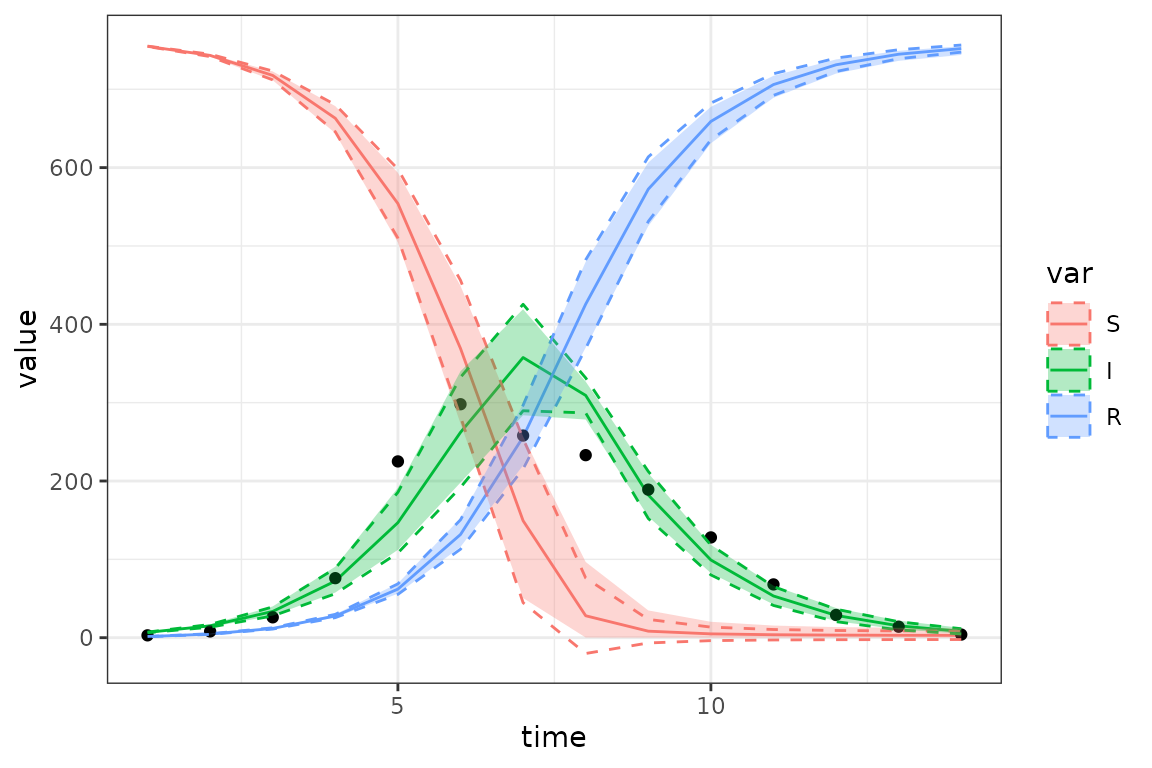

In this case the delta-method (dotted lines) and ensemble CIs (ribbons) are not that different (we can see that the ensemble CIs take care of the negative values in the CI); we certainly wouldn’t be badly misled by the delta method CIs in this case.

Since running the ensemble requires many (typically 500-1000) independent runs of the $report() method, you may want to do the computation in parallel. To do this, you can use any of the many available tools in R, for example: (parallel::parApply from base R, doParallel/foreach, future/furrr, etc.) For small models it may take longer to copy the TMBsimulator object over to all of the different workers than it takes to run the ensemble itself …

library(parallel)
ncores <- max(1, getOption("ncores", round(detectCores()/2)))
cl <- makeCluster(ncores)
clusterExport(cl = cl, "sir_simulator") ## may take a little while
sim2 <- parApply(cl = cl,
                 parvals, 1,
                 function(p) sir_simulator$report(p, .phases = "during")$value)
stopCluster(cl)
stopifnot(all.equal(sim_ensemble, sim2)) ## identical 

We can also compute prediction intervals via ensemble, by adding the appropriate amount of negative binomial noise to each simulation. However, it only makes sense to add this observation error to the I time series (if we had more than one observed time series we would probably want to estimate separate dispersion parameters for each series), so we’ll adapt the ensemble code to pick out only the I values before adding noise:

## negative binomial dispersion ('size') parameter
## (should be able to do this more nicely with a coef() method ...
nb_disp <- exp(fit$par[3])  
sim_ensemble2 <- apply(parvals, 1,
                       function(p) {
                           ## FIXME: misspelling '.phases' gives a 'wrong parameter length arg
                           s <- sir_simulator$report(p, .phases = "during")
                           v <- s$value[s$matrix == "I"]
                           ## force mean to be non-negative
                           ## we could also accept the warnings/NA values from negative predictions
                           rnbinom(length(v), mu = pmax(0, v), size = nb_disp)
                       })
I_ens <- data.frame(time = obs$time, var = "I", mk_quantiles(sim_ensemble2, suffix = "predens"))
## attach to existing data
res3 <- full_join(res2,  I_ens, by = c("time", "var"))
## plot
gg_ci3 <- (gg_base %+% res3) +
    geom_ribbon(aes(ymin = lwr_delta, ymax = upr_delta, colour = var), lty = 2, fill = NA) +
    geom_ribbon(aes(ymin = lwr_ens, ymax = upr_ens, colour = var), lty = 3, fill = NA) +
    geom_ribbon(aes(ymin = lwr_predens, ymax = upr_predens, fill = var), colour = NA, alpha = 0.3)
## suppress warnings about 'no non-missing args' [because we don't have *_predens vars for S and R]
suppressWarnings(
    print(gg_ci3)
    )

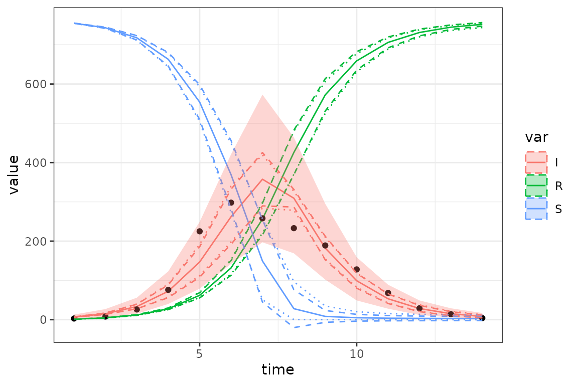
Unsurprisingly, the prediction intervals (ribbon) are much wider than the delta-method or ensemble-quantile (dashed and dotted lines) intervals.

Hamiltonian MC

under development

Since Markov chain Monte Carlo samples a wider range of the parameter space, it’s easier to get into numerical troubles - especially since we haven’t specified any prior distributions. We can mitigate these problems slightly by (1) specifying a random-number seed (so that at least any problems we have will be reproducible) and (2) specifying starting conditions rather than allowing Stan to pick them at random. Starting from the best-fit parameters works, but is conservative - ideally we want to make sure that our chains start from different points. Our second strategy is to use the best-fit parameters as a baseline, but jitter them randomly by ±40%.

library(tmbstan)
stan1 <- tmbstan(sir_simulator$ad_fun(), seed = 101, init  = "last.par.best")
#> Warning in tmbstan(sir_simulator$ad_fun(), seed = 101, init = "last.par.best"):
#> Re-cycling inits to match number of chains
init_fun <- function(jitter = 0.4) {
    p <- sir_simulator$ad_fun()$env$last.par.best
    p * runif(length(p), 1-jitter, 1+jitter)
}
stan2 <- tmbstan(sir_simulator$ad_fun(), init = init_fun, seed = 101)

broom.mixed::tidy(stan2, conf.int = TRUE)
#> # A tibble: 3 × 5
#>   term      estimate std.error conf.low conf.high
#>   <chr>        <dbl>     <dbl>    <dbl>     <dbl>
#> 1 params[1]    0.554    0.0324    0.498     0.627
#> 2 params[2]   -0.750    0.0700   -0.881    -0.613
#> 3 params[3]    2.54     0.558     1.37      3.59

(We should other diagnostics - check for divergent transitions, look at $\hat R$, traceplots, etc etc; see e.g. bayestestR::diagnostic_posterior(), bayeslot::mcmc_rank_overlay(), shinyStan … brief examples here.)

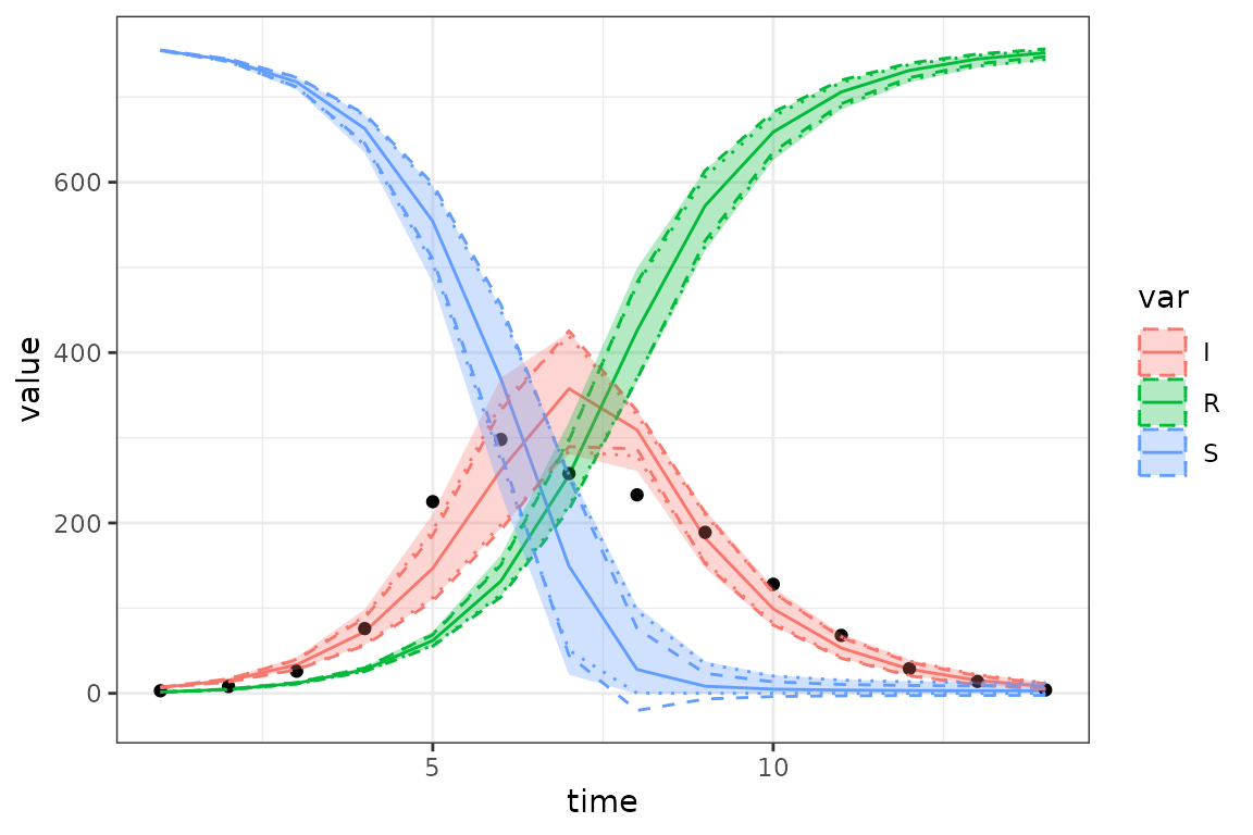
In this case the MCMC quantile credible intervals (ribbons) are pretty close to the delta-method and MVN ensemble CIs (shown as dotted lines) …

mcmc_pars <- as.data.frame(stan2, pars = "lp__", include = FALSE)
sim_mcmc <- apply(mcmc_pars, 1, function(p) sir_simulator$report(p, .phases = "during")$value) ## 48 x 1000
I_mcmc <- data.frame(time = obs$time, var = "I", mk_quantiles(sim_mcmc, suffix = "mcmc"))
## attach to existing data
res4 <- cbind(res3,  mk_quantiles(sim_mcmc, suffix = "mcmc"))
gg_ci4 <- (gg_base %+% res4) +
    geom_ribbon(aes(ymin = lwr_delta, ymax = upr_delta, colour = var), lty = 2, fill = NA) +
    geom_ribbon(aes(ymin = lwr_ens, ymax = upr_ens, colour = var), lty = 3, fill = NA) +
    geom_ribbon(aes(ymin = lwr_mcmc, ymax = upr_mcmc, fill = var), colour = NA, alpha = 0.3)
## suppress warnings about 'no non-missing args' [because we don't have *_predens vars for S and R]
suppressWarnings(
    print(gg_ci4)
    )

Alternative confidence intervals

As above, we can also get likelihood profile CIs …

ff <- sir_simulator$ad_fun()
class(ff) <- "TMB"
(broom.mixed::tidy(ff, conf.int = TRUE, conf.method = "profile")
    |> select(-c(type, std.error))
    |> mutate(term = drop_trans(coefnames(sir_simulator)))
    |> mutate(across(where(is.numeric), exp))
    |> as_tibble()
)

Irregular data; multiple data streams

For now we’re going to revert to the previous fake/simulated data. We’ll fit to both infection prevalence and number recovered, adding negative binomial observation noise and dropping 50% (approximately) of the observations at random

sir_simulator = mp_simulator(sir_spec
  , time_steps = 100
  , outputs = c("S", "I", "R")
  , default = list(N = 100, beta = 0.2, gamma = 0.1)
)
## `.phases = "during"` is important so that the number of observations matches the number of time steps
sir_results = sir_simulator$report(.phases = "during")
set.seed(101)
subsamp <- function(x, missprob = 0.5) { x[runif(length(x))<missprob] <- NA; x } 
sir_simdat <- (sir_results
    |> select(time, matrix, value)
    |> filter(matrix %in% c("I", "R"))
    |> pivot_wider(names_from = "matrix", values_from = "value")
    |> mutate(I_obs = subsamp(rnbinom(n(), mu = I, size = 4)),
              R_obs = subsamp(rnbinom(n(), mu = R, size = 8)))
    |> select(time, I_obs, R_obs)
)
## re-pivot for plotting purposes ...
plotdat <- sir_simdat |> pivot_longer(-time, names_to = "var", values_to = "count")
ggplot(plotdat, aes(time, count, colour = var)) + geom_point() +
    geom_smooth(method = "gam", method.args = list(family = quasipoisson))
#> `geom_smooth()` using formula = 'y ~ s(x, bs = "cs")'
#> Warning: Removed 91 rows containing non-finite outside the scale range
#> (`stat_smooth()`).
#> Warning: Removed 91 rows containing missing values or values outside the scale range
#> (`geom_point()`).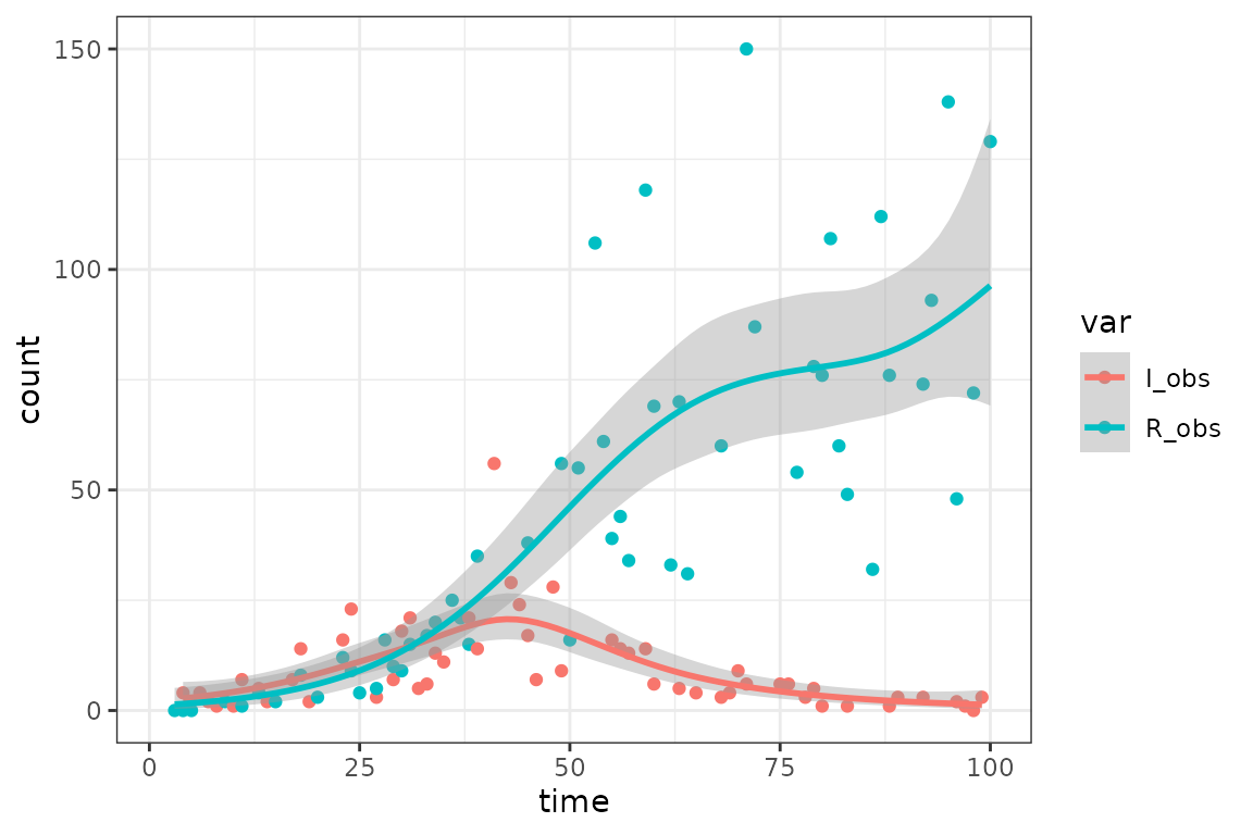

Numbers of samples with missing observations:

with(sir_simdat, table(I_missing=is.na(I_obs), R_missing=is.na(R_obs)))
#>          R_missing
#> I_missing FALSE TRUE
#>     FALSE    31   23
#>     TRUE     24   22

## won't work yet ... need more sophisticated obs/sim matching ...
# mk_calibrate(sir_simulator,
#              data = sir_simdat,
#              params = list(beta = 1, gamma = 0.5, I_disp = 1, R_disp = 1),
#              transforms = list(beta = "log", gamma = "log", I_disp = "log", R_disp = "log"),
#              exprs = list(log_lik ~ dnbinom(I_obs, I, I_disp) +
#                           dnbinom(R_obs, R, R_disp))
#              )

fixme:

• add more information from the original 1978-influenza article about probable starting date, duration, natural history?
• Comparison with fitode ?
• priors/regularization??
• (statistical) diagnostics? e.g. compute residuals, plot vs. time or vs fitted values, scale-location plot, etc. ?
• more CI stuff: importance sampling, Juul et al. functional ribbons, …
• intermediate examples
  • simple time-varying parameters
  • fitting multiple data streams (in progress)
  • irregularly sampled data (in progress)
  • estimate starting values
  • accumulators/differences: prevalence, deaths
  • forecasting/scenarios

‘Hello, World’ the hard way

This section explains what is going on under the hood in macpan2helpers::mk_calibrate()

Step 0: recreate the simulator

Since trying to add the same matrix to a simulator twice causes an error, we’ll create a new instance of the simulator:

sir_simulator = mp_simulator(sir_spec
  , time_steps = 100
  , outputs = c("S", "I", "R")
  , default = list(N = 100, beta = 0.2, gamma = 0.1)
)

Step 1: add observed data and slots for history etc.

While the files in the model library are sufficient to define a simulator, we now need to add more structure to the model object so we can do the calibration - specifically, both whatever observed data we want to compare against, and whatever new variables (“matrices”) and expressions we will evaluate to compute the goodness of fit (aka the loss function or objective function) of a particular set of parameters.

If we have a TMBSimulator object (i.e., sir_simulator in this example), the $add$matrices() method will add new variables to the space where the object has already stored the state variables, etc. (you use sir_simulator$matrix_names() to list the existing matrices, although this produces a long, scary list of internal variables that macpan2 has constructed)

Now we will use $add$matrices() to:

1. add observed data
2. declare a matrix storing the simulation history of variables to compare with observed data
3. declare a matrix to store the log-likelihood
4. specify which matrices to save and/or return in the report

sir_simulator$add$matrices(
  ## observed data
  I_obs = sir_prevalence$obs_val,
  ## simulated trajectory to compare with data
  I_sim = empty_matrix, 
  ## matrix to contain the log likelihood values at each time step
  log_lik = empty_matrix,
  ## need to save the simulation history of each of these matrices
  .mats_to_save = c("I_sim", "log_lik"),
  .mats_to_return = c("I_sim", "log_lik")
)

fixme: possibly comment that we could have added some of these objects up-front, in the definition files …

fixme: some examples show sir_simulator$print$matrix_dims() at this point. What is this good for/how do we interpret it?

Step 2: collect simulated values

Collect simulated values into matrices to be compared with data. the .at = Inf and .phase = "during" indicates that this expression should come at the end of the expressions evaluated during each iteration of the simulation loop.

Like $add$matrices(), $insert$expressions adds components to an existing TMBSimulator object - in this case, expressions that will be computed during the simulation. (In this example, since we set .phase = "during", the expressions will be computed at each time step.)

sir_simulator$insert$expressions(
  I_sim ~ I,
  .phase = "during",
  .at = Inf
)

fixme: what’s the best way to handle irregularly sampled data/match up with timestamps of observed data? (not for here, this should be a footnote or put in an ‘extra tricks’ section)

Step 3: set up and compute objective function

We will use the log (by default) of the Gaussian density of the observed I values with mean (i.e. predicted) value of the simulated I values (this is equivalent to least-squares estimation, with the added complication that we estimate the standard deviation explicitly rather than computing it from the residuals).

• Add the new parameter (standard deviation of the observed I distribution around the predicted I values)
• The rbind_time function gathers together the full simulation history of the I_sim matrix by binding together the rows at each iteration.

sir_simulator$add$matrices( I_sd = 1 )
sir_simulator$insert$expressions(
  log_lik ~ dnorm(I_obs, I_sim, I_sd),
  .phase = "after"
  )

Define the objective function (which will almost always be the sum of the negative log-likelihoods for each point):

sir_simulator$replace$obj_fn(~ -sum(log_lik))

Step 4: declare and/or transform parameters to be optimized, set starting values

• We could have postponed defining I_sd in the model until this step (fixme: right?), but it would have been confusing since we used it in the objective function.
• For parameters that are restricted to be positive, it is almost always best to estimate them on the log scale. This ensures that their values will always be non-negative (and positive unless the transformed values are negative and large enough in magnitude that exp(x) underflows to zero) and has other advantages in optimization (fixme: how much detail is needed here? Shrink scale of optimization, make parameter magnitudes ${\cal O}(1)$, make Wald estimation more reliable …)
• In practice we would often read the parameter starting values in from a CSV file (using read.csv from base R or readr::read_csv() from tidyverse), but here we can set up the data frame on the fly

sir_simulator$add$transformations(Log("I_sd"))
sir_simulator$add$transformations(Log("beta"))
params <- read.delim(sep = "|", header = TRUE,
                     text = "
mat       | default
log_I_sd  | 0
log_beta  | 1
")
sir_simulator$replace$params_frame(params)

Using $add_transformations(Log("var")) automatically adds a variable called log_var to the list of matrices.

Step 5: do the fit

It’s always a good idea to do some quick sanity checks on the objective function before you try to optimize: do you get finite values (for reasonable inputs)? Does changing the inputs change the returned value?

sir_simulator$objective(c(1,1))
#> [1] 776.0665
sir_simulator$objective(c(0,1))
#> [1] 4408.378

If you get error messages when running the objective function, sir_simulator$report() will help you debug by printing the expression that gave rise to the errors. sir_simulator$get$initial(<varname>) will print the initial values being used, while sir_simulator$current$params_frame() will print the full parameter data frame.

fixme: easier way to substitute a single parameter value? Way to modify starting conditions for optimizer on the fly? (Specifying start as an argument gives ‘formal argument “start” matched by multiple actual arguments’ – there should be a “replace if present” functionality)

fit <- sir_simulator$optimize$nlminb()

Measles Data – In-Progress

Here is a reasonably difficult problem – fit an SIR model to weekly measles incidence data from London UK over about six decades.

measles = read.csv(
  file.path(
    "https://raw.githubusercontent.com/davidearn/iidda/master/data",
    "meas_uk__lon_1944-94_wk/source-data/meas_uk__lon_1944-94_wk.csv"
  ),
  comment = "#"
)
measles$date = as.Date(sprintf(
  "%s-%s-%s", measles$year, measles$month, measles$day
))
plot(measles$date, measles$cases, type = "l")

We need to use a slightly extended version of the SIR specification that includes waning immunity.

sir_waning = mp_tmb_library("starter_models"
  , "sir_waning"
  , package = "macpan2"
)

We use radial basis functions to model time-variation in the transmission rate. We also make a variety of questionable assumptions (TODO: fix these), but the point at the moment is just to illustrate usage and provide a proof of concept.

d = 100
n = nrow(measles)
simulator = (sir_waning
  |> mp_simulator(
      time_steps = n
    , outputs = c("S", "I", "R", "infection")
    , default = list(
        N = 100000, I = 500
      , gamma = 0.2, phi = 0.01
      , X = rbf(n, d)
      , b = rnorm(d, sd = 0.01)
      , eta = empty_matrix
    )
  )
)
    
## radial basis function evaluations
simulator$insert$expressions(
    eta ~ gamma * exp(X %*% b)
  , .phase = "before"
  , .at = Inf
)
simulator$insert$expressions(
    beta ~ eta[time_step(1)] / clamp(S/N, 1/100)
  , .phase = "during"
  , .at = 1
)

Here is an example simulation from this model, before fitting to data.

simulated_incidence = filter(simulator$report(.phases = "during"), matrix == "infection")$value
plot(measles$date, simulated_incidence, type = "l", xlab = "time")

It looks nothing like the observed measles series, but illustrates the ability to generate complex incidence patterns not present in the simple SIR model without radial basis functions and waning immunity.

We modify the simulation object to be able to fit to the measles data.

simulator$add$matrices(
    reports = measles$cases
  , log_lik = empty_matrix
  , sim_reports = empty_matrix
)
simulator$insert$expressions(
    sim_reports ~ rbind_time(infection)
  , .phase = "after"
  , .at = Inf
)
simulator$replace$params(
  default = c(
      c(0.2, 0.01)
    , rep(0, d)
    , 500
  )
  , mat = c(
      c("gamma", "phi")
    , rep("b", d)
    , "I"
  )
  , row = c(
      rep(0, 2L)
    , seq_len(d) - 1L
    , 0L
  )
)
simulator$replace$obj_fn(~ - sum(dpois(reports, sim_reports)))

The optimization takes quite a few minutes, and still doesn’t converge in 10000 function evaluations.

simulator$optimize$nlminb(control = list(eval.max = 10000, iter.max = 10000, trace = 10))

simulator$optimization_history$get()[[3]]  ## the 3 is there because we tried two other times

Here the red data are fitted and black observed.

simulated_incidence = filter(simulator$report(.phases = "during"), matrix == "incidence")$value
plot(measles$date, measles$cases, xlab = "time", type = "l")
lines(measles$date, simulated_incidence, col = 2)

Not a perfect fit, but not bad for now (TODO: work on this, without papering over the real challenges).

Challenging Logistic Variation in Transmission Rate

Here we consider the problem of fitting an SIR model to a simulated dataset from this model, such that the simulations pose challenges to the fitting machinery.

sir_simulator = mp_simulator(sir_spec
  , time_steps = 100
  , outputs = c("S", "I", "R")
  , default = list(
      N = 100000, I = 500
    , beta = 0.2, gamma = 0.2
  )
)

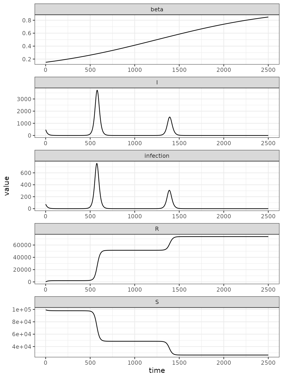
Our simulation model includes a logistically time-varying transmission rate.

n = 2500
set.seed(1L)
simulator = (sir_spec
  |> mp_simulator(
      time_steps = n
    , outputs = c("S", "I", "R", "beta", "infection")
    , default = list(
        N = 100000, I = 500
      , beta = 0.2, gamma = 0.2
      , X = cbind(1, scale(seq_len(n)))
      , b = c(0, 1)
      , beta_values = empty_matrix
    )
  )
)
simulator$insert$expressions(
    beta_values ~ 1 / (1 + exp(-X %*% b))
  , .phase = "before"
  , .at = Inf
)
simulator$insert$expressions(
    beta ~ beta_values[time_step(1)]
  , .phase = "during"
  , .at = 1
)
simulator$replace$params(
    default = c(0, 1)
  , mat = rep("b", 2)
  , row = 0:1
)

set.seed(5L)
sims = mp_trajectory(simulator)
(sims
  |> rename(variable = matrix)
  |> ggplot()
  + facet_wrap(~ variable, ncol = 1, scales = 'free')
  + geom_line(aes(time, value))
)

Fitting to the simulation data, manages to converge, but to the wrong value.

set.seed(3L) ## different seeds do result in convergence on the correct value
reports = filter(sims, matrix == "infection")$value
simulator$add$matrices(reports = reports, report_sim = empty_matrix)
simulator$insert$expressions(
    report_sim ~ rbind_time(infection)
  , .phase = "after"
  , .at = Inf
)
simulator$replace$obj_fn(~ -sum(dpois(reports, report_sim)))
simulator$replace$params(
    default = rnorm(2L) ## random starting values for the optimizer
  , mat = rep("b", 2)
  , row = 0:1
)
simulator$optimize$nlminb()
#> outer mgc:  11268970 
#> outer mgc:  7215054 
#> outer mgc:  3087372 
#> outer mgc:  3522804 
#> outer mgc:  470268.8 
#> outer mgc:  802897.8 
#> outer mgc:  133686.6 
#> outer mgc:  4449.854 
#> outer mgc:  5.260259 
#> outer mgc:  7.984454e-06
#> $par
#>     params     params 
#> -1.0929130  0.1633477 
#> 
#> $objective
#> [1] 326073.6
#> 
#> $convergence
#> [1] 0
#> 
#> $iterations
#> [1] 9
#> 
#> $evaluations
#> function gradient 
#>       12       10 
#> 
#> $message
#> [1] "both X-convergence and relative convergence (5)"
simulator$current$params_frame()
#>   par_id mat row col    default    current
#> 1      0   b   0   0 -0.9619334 -1.0929130
#> 2      1   b   1   0 -0.2925257  0.1633477
fitted_incidence = (simulator$current$params_vector()
  |> simulator$report()
  |> filter(matrix == "infection")
  |> pull(value)
)
plot(reports, type = "l")
lines(fitted_incidence, col = 2)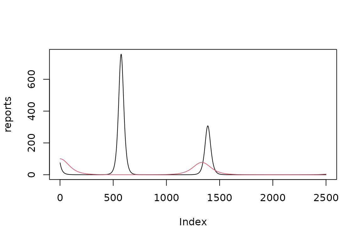

The fit is not good! Even though we are fitting the extact noiseless data generating model, so why is the fit not good? To find out we plot the likelihood surface with arrows representing the magnitude and direction of the down-hill gradient towards the optimum. Notice the very flat gradient in the direction along the valley containing the optimum at $(0, 1)$. The gradient is pointing towards the valley but not along it. I do not understand why.

make_liksurf <- function(lwr = c(-1, 0), upr = c(1, 2),
                         n = c(41, 41)) {
    lik_surf = expand.grid(
        intercept_parameter = seq(from = lwr[1], to = upr[1], 
                                  length.out = n[1]),
        slope_parameter = seq(from = lwr[2], to = upr[2],
                              length.out = n[2])
    )
    gr = t(apply(lik_surf, 1, simulator$gradient))
    lik_surf$z = apply(lik_surf, 1, simulator$objective)
    gr = 0.1 * gr / max(abs(gr))
    lik_surf$gx = gr[,1]
    lik_surf$gy = gr[,2]
    return(lik_surf)
}
lik_surf <- make_liksurf()

mk_plot <- function(dd, arrows = TRUE, contours = TRUE,
                    arrow_len = 0.05,
                    cbrks = (1:10)*1e5) {
    gg0 <- (ggplot(dd, aes(intercept_parameter, slope_parameter))
        + geom_tile(aes(fill = z))
        + theme_bw()
        + scale_x_continuous(expand = c(0,0))
        + scale_y_continuous(expand = c(0,0))
        + annotate(geom = "point", x = 0, y = 1, colour = "yellow", size = 2,
                   pch = 16)
        + scale_fill_continuous(trans = "log10")

    )
    if (contours) {
        gg0 <- gg0 + geom_contour(aes(z = z), colour = "red",
                                  breaks = cbrks)
    }
    if (arrows) {
        gg0 <- gg0 + geom_segment(
                         data = dd[seq(nrow(dd)) %% 5 == 0 , ],
                         aes(
                             xend = intercept_parameter - gx, 
                             yend = slope_parameter - gy
                         ), 
                         arrow = arrow(length = unit(arrow_len, "inches")), 
                         colour = 'white'
                     )
    }
    gg0
}
print(mk_plot(lik_surf))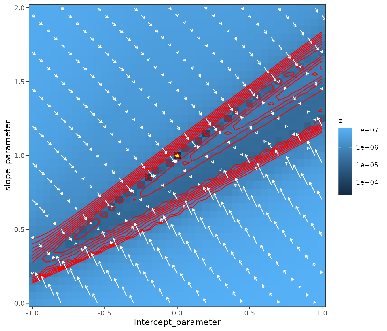

lik_surf2 <- make_liksurf(lwr = c(-0.1, 0.9), upr = c(0.1, 1.1))
print(mk_plot(lik_surf2, arrows = FALSE, cbrks = 1e4*(1:10)))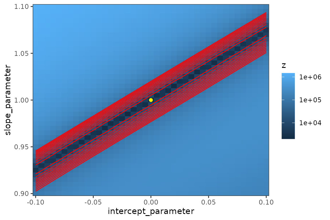

Explore more carefully:

make_mat <- function(x) {
  with(x, matrix(z, sqrt(length(z)),
            dimnames = list(intercept = unique(intercept_parameter),
                            slope = unique(slope_parameter)))
       )
}
library(rgl)
z1 <- make_mat(lik_surf)
persp3d(as.numeric(rownames(z)), as.numeric(colnames(z)), log10(z),
        col = "gray")
z2 <- make_mat(lik_surf2)
persp3d(as.numeric(rownames(z2)), as.numeric(colnames(z2)), log10(z2),
        col = "gray")

fixme: what causes spikiness along the ridge? Add points where each optimization attempt stopped?

experimental: working with DEoptim (haven’t included yet because I don’t want to have to Suggest: DEoptim …

library(DEoptim)
set.seed(101)
fit <- DEoptim(simulator$objective, lower = rep(-10, 2), upper = rep(10, 2))
fitted_incidence = (simulator$ad_fun()$env$last.par.best
    |> simulator$report()
    |> filter(matrix == "infection")
    |> pull(value)
)
plot(reports, type = "l")
lines(fitted_incidence, col = 2)

• fixme: also add multi-start example (i.e. less fancy than DEoptim, suitable for surfaces like this one that are multimodal but smooth (ref. Raue et al. “Lessons Learned from Quantitative Dynamical Modeling in Systems Biology” 2013)?)

• fixme: warning that $current$params_vector() is mutable/unreliable. Extractor for $ad_fun()$env$last.par.best (or equivalently for the optim fit)?

• fixme: add (abbreviated) sessionInfo output? (Package versions?)