Fitting to Real Data • macpan2

The vignette("quickstart") and vignette("calibration") articles work with simulated data, but it is more interesting to fit models to real data. The International Infectious Disease Data Archive (IIDDA) is a useful place to look for incidence, mortality, and population data for illustrating macpan2. This archive contains data from this data digitization project, which we will use here. What we find is that with real data, even with relatively simple models and calibration problems, issues can arise that require careful thought.

Setup

As usual we need the following packages. If you don’t have them, please get them in the usual way (i.e. using install.packages).

library(macpan2)
library(dplyr)
library(ggplot2)
library(broom.mixed)

In addition, we need the iidda.api package.

if (!require(iidda.api)) {
  repos = c(
      "https://canmod.r-universe.dev"
    , "https://cran.r-project.org"
  )
  install.packages("iidda.api", repos = repos)
}
api_hook = iidda.api::ops_staging

And we set a few options for convenience.

options(iidda_api_msgs = FALSE, macpan2_verbose = FALSE)

One Scarlet Fever Outbreak in Ontario

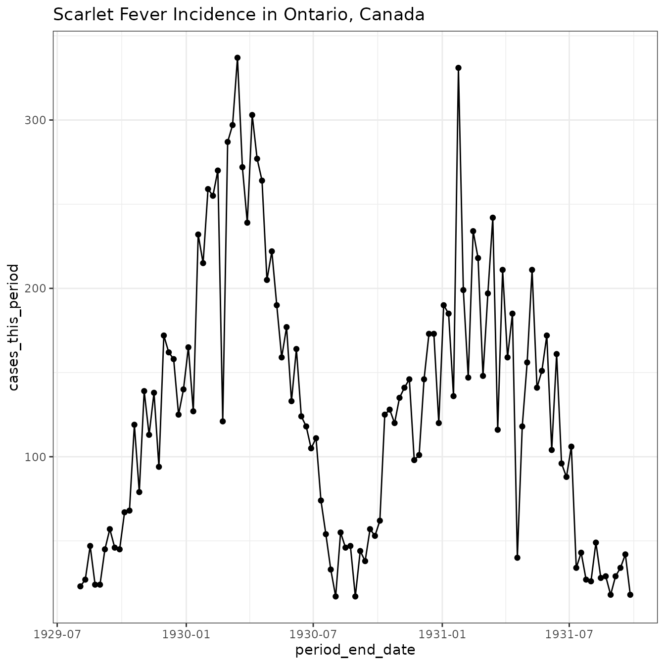
The following code will pull data for a single scarlet fever outbreak in Ontario that ended in 1930.

scarlet_fever_ontario = api_hook$filter(resource_type = "CANMOD CDI"
  , iso_3166_2 = "CA-ON"  ## get ontario data
  , time_scale = "wk"  ## weekly incidence data only 
  , disease = "scarlet-fever"
  
  # get data between 1929-08-01 and 1930-10-01
  , period_end_date = "1929-08-01..1930-10-01"
)
print(scarlet_fever_ontario)
#> # A tibble: 61 × 19
#>    iso_3166 iso_3166_2 location location_type period_start_date period_end_date
#>    <chr>    <chr>      <chr>    <chr>         <date>            <date>         
#>  1 CA       CA-ON      ONT.     province      1929-07-28        1929-08-03     
#>  2 CA       CA-ON      ONT.     province      1929-08-04        1929-08-10     
#>  3 CA       CA-ON      ONT.     province      1929-08-11        1929-08-17     
#>  4 CA       CA-ON      ONT.     province      1929-08-18        1929-08-24     
#>  5 CA       CA-ON      ONT.     province      1929-08-25        1929-08-31     
#>  6 CA       CA-ON      ONT.     province      1929-09-01        1929-09-07     
#>  7 CA       CA-ON      ONT.     province      1929-09-08        1929-09-14     
#>  8 CA       CA-ON      ONT.     province      1929-09-15        1929-09-21     
#>  9 CA       CA-ON      ONT.     province      1929-09-22        1929-09-28     
#> 10 CA       CA-ON      ONT.     province      1929-09-29        1929-10-05     
#> # ℹ 51 more rows
#> # ℹ 13 more variables: period_mid_date <date>, days_this_period <dbl>,
#> #   time_scale <chr>, disease <chr>, nesting_disease <chr>,
#> #   historical_disease_family <chr>, historical_disease <chr>,
#> #   historical_disease_subclass <chr>, dataset_id <chr>,
#> #   original_dataset_id <chr>, cases_this_period <dbl>, population <dbl>,
#> #   population_reporting <dbl>

This is what the data looks like.

(scarlet_fever_ontario
  |> ggplot(aes(period_mid_date, cases_this_period))
  + geom_line() + geom_point()
  + ggtitle("Scarlet Fever Incidence in Ontario, Canada")
  + theme_bw()
)

SIR Model

We will begin by pulling the simple sir model from the model library.

sir = mp_tmb_library("starter_models", "sir", package = "macpan2")
print(sir)
#> ---------------------
#> Default values:
#> ---------------------
#>  matrix row col value
#>    beta           0.2
#>   gamma           0.1
#>       N         100.0
#>       I           1.0
#>       R           0.0
#> 
#> ---------------------
#> Before the simulation loop (t = 0):
#> ---------------------
#> 1: S ~ N - I - R
#> 
#> ---------------------
#> At every iteration of the simulation loop (t = 1 to T):
#> ---------------------
#> 1: mp_per_capita_flow(from = "S", to = "I", rate = infection ~ I * 
#>      beta/N)
#> 2: mp_per_capita_flow(from = "I", to = "R", rate = recovery ~ gamma)

Modify Model for Reality

Once we take any library model off the shelf we need to modify it a bit to be more realistic. We do this with the mp_tmb_insert() function, which inserts new default values and model expressions.

We first change the population size to the population of Ontario at the time.

sf_sir = mp_tmb_insert(sir
  , default = list(N = median(scarlet_fever_ontario$population))
)

Second, our SIR model assumes that all of the cases are recorded in the data, but this is not realistic. We therefore modify the model to include under-reporting, by creating a case reports variable that is given by the product of incidence (i.e. weekly infection rate) and a reporting probability.

sf_sir = mp_tmb_insert(sf_sir
    ## insert this expression ...
  , expressions = list(reports ~ infection * report_prob)
    
    ## at the end (i.e. Infinity) of the expressions evaluated
    ## 'during' each iteration of the simulation loop ...
  , at = Inf  
  , phase = "during"
  
    ## add a new default value for the reporting probability
  , default = list(report_prob = 1/300)
)

Here we can print out the modified model to see if our changes were made successfully.

print(sf_sir)
#> ---------------------
#> Default values:
#> ---------------------
#>       matrix row col        value
#>         beta         2.000000e-01
#>        gamma         1.000000e-01
#>            N         3.392636e+06
#>            I         1.000000e+00
#>            R         0.000000e+00
#>  report_prob         3.333333e-03
#> 
#> ---------------------
#> Before the simulation loop (t = 0):
#> ---------------------
#> 1: S ~ N - I - R
#> 
#> ---------------------
#> At every iteration of the simulation loop (t = 1 to T):
#> ---------------------
#> 1: mp_per_capita_flow(from = "S", to = "I", rate = infection ~ I * 
#>      beta/N)
#> 2: mp_per_capita_flow(from = "I", to = "R", rate = recovery ~ gamma)
#> 3: reports ~ infection * report_prob

Preparing the Data

The first step in preparing data for macpan2 is to simulate from the model that you are considering. Here we simulate the "reports" variable because it corresponds to the reported incidence (the number of new cases per time-step, which in our case is one week, multiplied by a reporting probability).

sir_simulator = mp_simulator(sf_sir
  , time_steps = 5
  , outputs = "reports"
)
head(mp_trajectory(sir_simulator))
#>    matrix time row col        value
#> 1 reports    1   0   0 0.0006666665
#> 2 reports    2   0   0 0.0007333330
#> 3 reports    3   0   0 0.0008066662
#> 4 reports    4   0   0 0.0008873327
#> 5 reports    5   0   0 0.0009760658

The next step is to get our data into a format that is compatible with the format of these simulations. In particular, we need matrix, time, and value columns. We can omit the row and col columns, because all of the ‘matrices’ in the model are 1-by-1 scalars.

observed_data = (scarlet_fever_ontario
  ## select the variables to be modelled -- a time-series of case reports.
  |> select(period_end_date, cases_this_period)
  
  ## change the column headings so that they match the columns
  ## in the simulated trajectories.
  |> mutate(matrix = "reports")
  |> rename(value = cases_this_period)
  
  ## create a `time` column with the time-step IDs that will correspond
  ## to the time-steps in the simulation. this column heading also 
  ## must match the column with the time-steps in the simulated trajectories
  |> mutate(time = seq_along(period_end_date))
)
print(head(observed_data))
#> # A tibble: 6 × 4
#>   period_end_date value matrix   time
#>   <date>          <dbl> <chr>   <int>
#> 1 1929-08-03         23 reports     1
#> 2 1929-08-10         27 reports     2
#> 3 1929-08-17         47 reports     3
#> 4 1929-08-24         24 reports     4
#> 5 1929-08-31         24 reports     5
#> 6 1929-09-07         45 reports     6

Set up the Optimizer

Now we can create an object that can be calibrated.

sir_cal = mp_tmb_calibrator(
    spec = sf_sir
  , data = observed_data
  
  ## name the trajectory variable, with a name that
  ## is the same in both the spec and the data
  , traj = "reports"  
  
  ## fit the following parameters
  , par = c("beta", "gamma", "I", "report_prob")
)

Here we assert that we will fit beta, gamma, (the initial value of) I, and report_prob. Note that we can only choose to fit parameters in the default list of the model spec. In particular, I is in the default list because the model requires the initial number of infectious individuals, whereas S is not because it is derived before the simulation loop as S ~ N - I - R.

print(sf_sir)
#> ---------------------
#> Default values:
#> ---------------------
#>       matrix row col        value
#>         beta         2.000000e-01
#>        gamma         1.000000e-01
#>            N         3.392636e+06
#>            I         1.000000e+00
#>            R         0.000000e+00
#>  report_prob         3.333333e-03
#> 
#> ---------------------
#> Before the simulation loop (t = 0):
#> ---------------------
#> 1: S ~ N - I - R
#> 
#> ---------------------
#> At every iteration of the simulation loop (t = 1 to T):
#> ---------------------
#> 1: mp_per_capita_flow(from = "S", to = "I", rate = infection ~ I * 
#>      beta/N)
#> 2: mp_per_capita_flow(from = "I", to = "R", rate = recovery ~ gamma)
#> 3: reports ~ infection * report_prob

Run the Optimization

sir_opt = mp_optimize(sir_cal)
#> Warning in (function (start, objective, gradient = NULL, hessian = NULL, :
#> NA/NaN function evaluation
#> Warning in (function (start, objective, gradient = NULL, hessian = NULL, :
#> NA/NaN function evaluation
#> Warning in (function (start, objective, gradient = NULL, hessian = NULL, :
#> NA/NaN function evaluation

Not off to a good start. Those warnings are not necessarily bad, but they might get us thinking.

Examine the fit

print(sir_opt)
#> $par
#>     params     params     params     params 
#> 29.0058616 28.8891098  2.6406276  0.2895818 
#> 
#> $objective
#> [1] 424.55
#> 
#> $convergence
#> [1] 1
#> 
#> $iterations
#> [1] 118
#> 
#> $evaluations
#> function gradient 
#>      200      119 
#> 
#> $message
#> [1] "function evaluation limit reached without convergence (9)"

OK, things are not great. The convergence code is 1, indicating that the model did not converge (convergence == 0 is good). Examining the parameter estimates, which are stored internally in the calibrator object, things get worse.

mp_tmb_coef(sir_cal, conf.int = TRUE)
#>       term         mat row col     default  type   estimate std.error
#> 1   params        beta   0   0 0.200000000 fixed 29.0058616 17.616797
#> 2 params.1       gamma   0   0 0.100000000 fixed 28.8891098 17.616948
#> 3 params.2           I   0   0 1.000000000 fixed  2.6406276  3.204148
#> 4 params.3 report_prob   0   0 0.003333333 fixed  0.2895818  0.175993
#>     conf.low  conf.high
#> 1 -5.5224261 63.5341493
#> 2 -5.6394732 63.4176929
#> 3 -3.6393864  8.9206416
#> 4 -0.0553582  0.6345218

That doesn’t look right! Those are very high beta and gamma values, and the confidence intervals are enormous and overlap zero.

But the model fit doesn’t look all that bad.

fitted_data = mp_trajectory_sd(sir_cal, conf.int = TRUE)
(observed_data
  |> ggplot()
  + geom_point(aes(time, value))
  + geom_line(aes(time, value)
    , data = fitted_data
  )
  + geom_ribbon(aes(time, ymin = conf.low, ymax = conf.high)
    , data = fitted_data
    , alpha = 0.2
    , colour = "red"
  )
  + theme_bw()
  + facet_wrap(~matrix, ncol = 1, scales = "free")
)

What is going on? Can we modify this model and/or fitting procedure to get both reasonable parameter estimates and a reasonable trajectory?

Fixing the Optimization Problem

One way to address the lack of convergence of the optimizer is to assess the degree to which the parameter estimates are biologically reasonable. Take the recovery rate, which is estimated as gamma ~ 26.5 per time-step. Given that a time-step is one week in this model, this estimate implies that individuals recover from scarlet fever in 1/26.5 weeks – much less than a day. A quick search suggests to me that this recovery rate is not reasonable for scarlet fever, and that a rough guess that the infectious stage lasts one week is much more plausible than 1/26.5 weeks. Now look at the transmission rate, beta. It is also estimated to be pretty large, but what is more interesting is the large standard errors for both beta and gamma. These standard errors suggest that the estimates are not precise. However, the estimated correlation between beta and gamma is very close to 1, suggesting that many values for these parameters would fit the data well as long as they are both of similar magnitude.

mp_tmb_fixef_cov(sir_cal) |> cov2cor()
#>                   beta      gamma          I report_prob
#> beta         1.0000000  1.0000000 -0.9997652   0.9995361
#> gamma        1.0000000  1.0000000 -0.9997636   0.9995384
#> I           -0.9997652 -0.9997636  1.0000000  -0.9989125
#> report_prob  0.9995361  0.9995384 -0.9989125   1.0000000

This diagnosis, if correct, suggests that the data are not sufficiently informative to identify values for both beta and gamma. Resolving such identifiability issues is often best done by introducing prior information, such as our rough guess that gamma is close to 1. The simplest way to include such prior information is to move gamma out of the pars argument to mp_tmb_calibrator and into the default argument, as below.

sir_cal_assume_gamma = mp_tmb_calibrator(
    spec = sf_sir
  , data = observed_data
  
  ## name the trajectory variable, with a name that
  ## is the same in both the spec and the data
  , traj = "reports"  
  
  ## fit the following parameters
  , par = c("beta", "I", "report_prob")
  , default = list(gamma = 1)
)

This calibration specification does not try to jointly fit both beta and gamma, but rather fits only beta while assuming that gamma = 1.

sir_opt_assume_gamma = mp_optimize(sir_cal_assume_gamma)
#> Warning in (function (start, objective, gradient = NULL, hessian = NULL, :
#> NA/NaN function evaluation
#> Warning in (function (start, objective, gradient = NULL, hessian = NULL, :
#> NA/NaN function evaluation
#> Warning in (function (start, objective, gradient = NULL, hessian = NULL, :
#> NA/NaN function evaluation
#> Warning in (function (start, objective, gradient = NULL, hessian = NULL, :
#> NA/NaN function evaluation
#> Warning in (function (start, objective, gradient = NULL, hessian = NULL, :
#> NA/NaN function evaluation

print(sir_opt_assume_gamma)
#> $par
#>       params       params       params 
#> 1.122440e+00 1.669046e+03 1.123683e-02 
#> 
#> $objective
#> [1] 426.6981
#> 
#> $convergence
#> [1] 0
#> 
#> $iterations
#> [1] 81
#> 
#> $evaluations
#> function gradient 
#>      124       81 
#> 
#> $message
#> [1] "both X-convergence and relative convergence (5)"

More warnings, but now the optimizer converges. And the standard errors in the coefficient table and fixed effect correlations seem more plausible.

mp_tmb_coef(sir_cal_assume_gamma)
#>       term         mat row col     default  type     estimate    std.error
#> 1   params        beta   0   0 0.200000000 fixed 1.122440e+00  0.001789219
#> 2 params.1           I   0   0 1.000000000 fixed 1.669046e+03 50.635015008
#> 3 params.2 report_prob   0   0 0.003333333 fixed 1.123683e-02  0.000192139

mp_tmb_fixef_cov(sir_cal_assume_gamma) |> cov2cor()
#>                   beta          I report_prob
#> beta         1.0000000 -0.8155308  -0.7603637
#> I           -0.8155308  1.0000000   0.5966437
#> report_prob -0.7603637  0.5966437   1.0000000

And the fit looks similar to the four-parameter model, which is consistent with our diagnosis of non-identifiability.

fitted_data = mp_trajectory_sd(sir_cal_assume_gamma, conf.int = TRUE)
(observed_data
  |> ggplot()
  + geom_point(aes(time, value))
  + geom_line(aes(time, value)
    , data = fitted_data
  )
  + geom_ribbon(aes(time, ymin = conf.low, ymax = conf.high)
    , data = fitted_data
    , alpha = 0.2
    , colour = "red"
  )
  + theme_bw()
  + facet_wrap(~matrix, ncol = 1, scales = "free")
)

Caution: Ben, what is that paper that you always recommend about being careful when prior information is included without prior uncertainty? This one (Elderd, Dukic, and Dwyer 2006)

Learning the Functional form of Time Variation in Transmission (New!)

Let’s get a bit more data to see two seasons.

scarlet_fever_ontario = api_hook$filter(resource_type = "CANMOD CDI"
  , iso_3166_2 = "CA-ON"  ## get ontario data
  , time_scale = "wk"  ## weekly incidence data only 
  , disease = "scarlet-fever"
  
  # get data between 1929-08-01 and 1931-10-01
  , period_end_date = "1929-08-01..1931-10-01"  
)
(scarlet_fever_ontario
  |> ggplot(aes(period_mid_date, cases_this_period))
  + geom_line() + geom_point()
  + ggtitle("Scarlet Fever Incidence in Ontario, Canada")
  + theme_bw()
)

observed_data = (scarlet_fever_ontario
  ## select the variables to be modelled -- a time-series of case reports.
  |> select(period_end_date, cases_this_period)
  
  ## change the column headings so that they match the columns
  ## in the simulated trajectories.
  |> mutate(matrix = "reports")
  |> rename(value = cases_this_period)
  
  ## create a `time` column with the time-step IDs that will correspond
  ## to the time-steps in the simulation. this column heading also 
  ## must match the column with the time-steps in the simulated trajectories
  |> mutate(time = seq_along(period_end_date))
)
print(head(observed_data))
#> # A tibble: 6 × 4
#>   period_end_date value matrix   time
#>   <date>          <dbl> <chr>   <int>
#> 1 1929-08-03         23 reports     1
#> 2 1929-08-10         27 reports     2
#> 3 1929-08-17         47 reports     3
#> 4 1929-08-24         24 reports     4
#> 5 1929-08-31         24 reports     5
#> 6 1929-09-07         45 reports     6

Prepare to fit to the data. We make a function so that we can easily update the dimension of the radial basis.

make_rbf_calibrator = function(dimension) {
  mp_tmb_calibrator(
      spec = sf_sir
    , data = observed_data
    , traj = "reports"  
    
    ## -----------------------------
    ## this is the key bit
    , tv = mp_rbf("beta", dimension)
    ## -----------------------------
    
    , par = c("gamma", "I", "report_prob")
  )
}

And it is also convenient to make a function for plotting the results

plot_fit = function(cal_object) {
  fitted_data = mp_trajectory_sd(cal_object, conf.int = TRUE)
  (observed_data
    |> ggplot()
    + geom_point(aes(time, value))
    + geom_line(aes(time, value)
      , data = fitted_data
      , colour = "red"
    )
    + geom_ribbon(aes(time, ymin = conf.low, ymax = conf.high)
      , data = fitted_data
      , alpha = 0.2
      , colour = "red"
    )
    + theme_bw()
  )
}

Now we try fitting for a number of different dimensions.

sir_cal = make_rbf_calibrator(dimension = 1)
mp_optimize(sir_cal)
#> $par
#>     params     params     params     params 
#>  1.1161463 88.4704036  0.8660326  0.1269302 
#> 
#> $objective
#> [1] 2757.747
#> 
#> $convergence
#> [1] 1
#> 
#> $iterations
#> [1] 133
#> 
#> $evaluations
#> function gradient 
#>      200      133 
#> 
#> $message
#> [1] "function evaluation limit reached without convergence (9)"

plot_fit(sir_cal)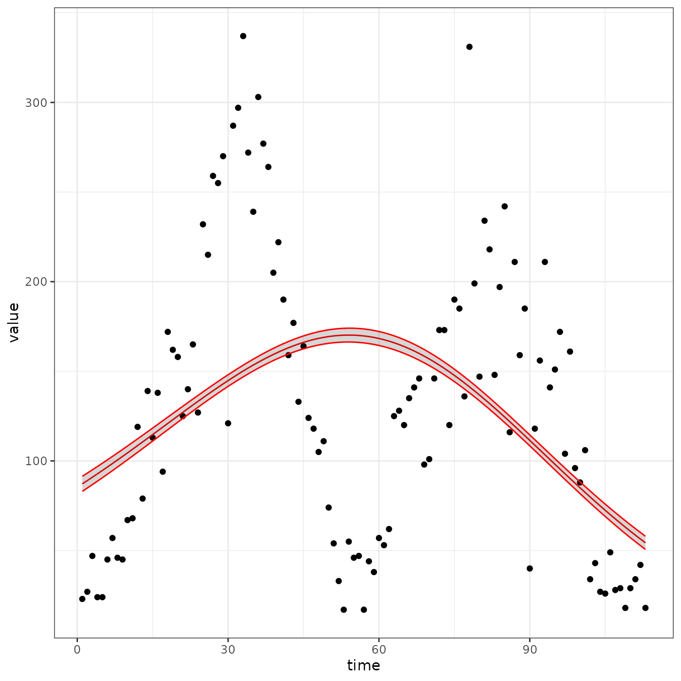

sir_cal = make_rbf_calibrator(dimension = 2)
mp_optimize(sir_cal)
#> $par
#>      params      params      params      params      params 
#>  0.03614755 37.88296337 13.70413466 -1.73565077 -3.36834735 
#> 
#> $objective
#> [1] 2769.557
#> 
#> $convergence
#> [1] 1
#> 
#> $iterations
#> [1] 119
#> 
#> $evaluations
#> function gradient 
#>      200      120 
#> 
#> $message
#> [1] "function evaluation limit reached without convergence (9)"

plot_fit(sir_cal)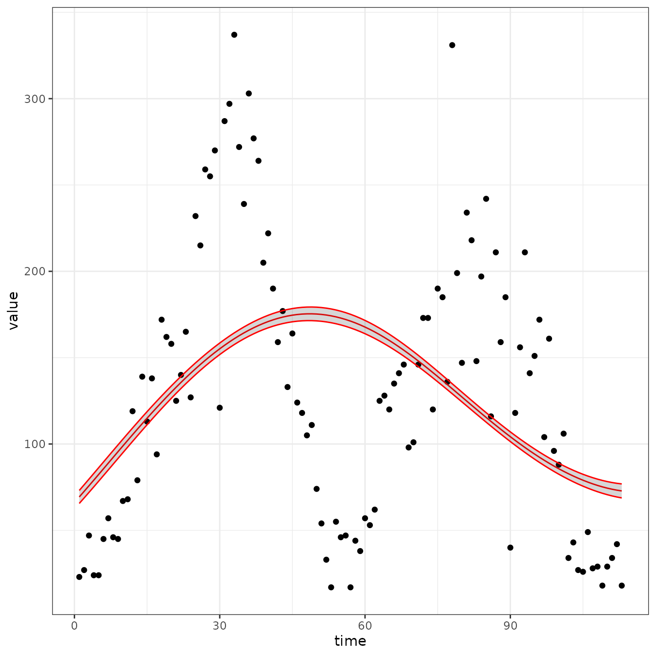

sir_cal = make_rbf_calibrator(dimension = 3)
mp_optimize(sir_cal)
#> Warning in (function (start, objective, gradient = NULL, hessian = NULL, :
#> NA/NaN function evaluation
#> Warning in (function (start, objective, gradient = NULL, hessian = NULL, :
#> NA/NaN function evaluation
#> Warning in (function (start, objective, gradient = NULL, hessian = NULL, :
#> NA/NaN function evaluation
#> Warning in (function (start, objective, gradient = NULL, hessian = NULL, :
#> NA/NaN function evaluation
#> $par
#>        params        params        params        params        params 
#>  7.445217e-01  6.323353e+03  5.707895e-03 -1.592204e-01 -4.668529e-02 
#>        params 
#>  9.091554e-01 
#> 
#> $objective
#> [1] 1249.741
#> 
#> $convergence
#> [1] 0
#> 
#> $iterations
#> [1] 70
#> 
#> $evaluations
#> function gradient 
#>       96       71 
#> 
#> $message
#> [1] "relative convergence (4)"

plot_fit(sir_cal)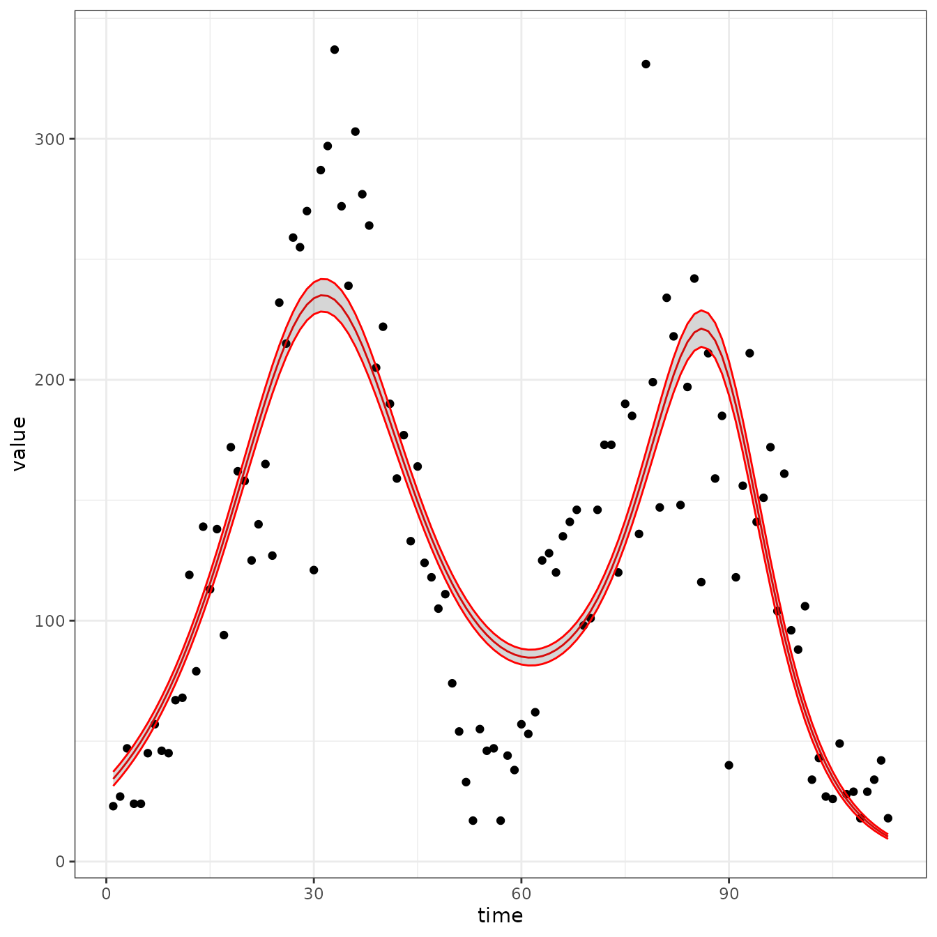

sir_cal = make_rbf_calibrator(dimension = 4)
mp_optimize(sir_cal)
#> Warning in (function (start, objective, gradient = NULL, hessian = NULL, :
#> NA/NaN function evaluation
#> Warning in (function (start, objective, gradient = NULL, hessian = NULL, :
#> NA/NaN function evaluation
#> Warning in (function (start, objective, gradient = NULL, hessian = NULL, :
#> NA/NaN function evaluation
#> $par
#>       params       params       params       params       params       params 
#>   1.30734342 106.01354219   0.07401727   0.42630267  -0.06942185   0.35248532 
#>       params 
#>   0.01001478 
#> 
#> $objective
#> [1] 1228.817
#> 
#> $convergence
#> [1] 1
#> 
#> $iterations
#> [1] 116
#> 
#> $evaluations
#> function gradient 
#>      200      116 
#> 
#> $message
#> [1] "function evaluation limit reached without convergence (9)"

plot_fit(sir_cal)

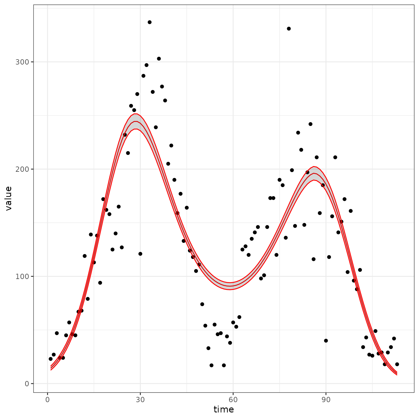
sir_cal = make_rbf_calibrator(dimension = 5)
mp_optimize(sir_cal)
#> $par
#>      params      params      params      params      params      params 
#>  0.02023712 23.88310851 23.63162276 -3.47579664  1.65114417 -5.44649398 
#>      params      params 
#>  1.86159848 -5.85211557 
#> 
#> $objective
#> [1] 1039.075
#> 
#> $convergence
#> [1] 1
#> 
#> $iterations
#> [1] 120
#> 
#> $evaluations
#> function gradient 
#>      200      120 
#> 
#> $message
#> [1] "function evaluation limit reached without convergence (9)"

plot_fit(sir_cal)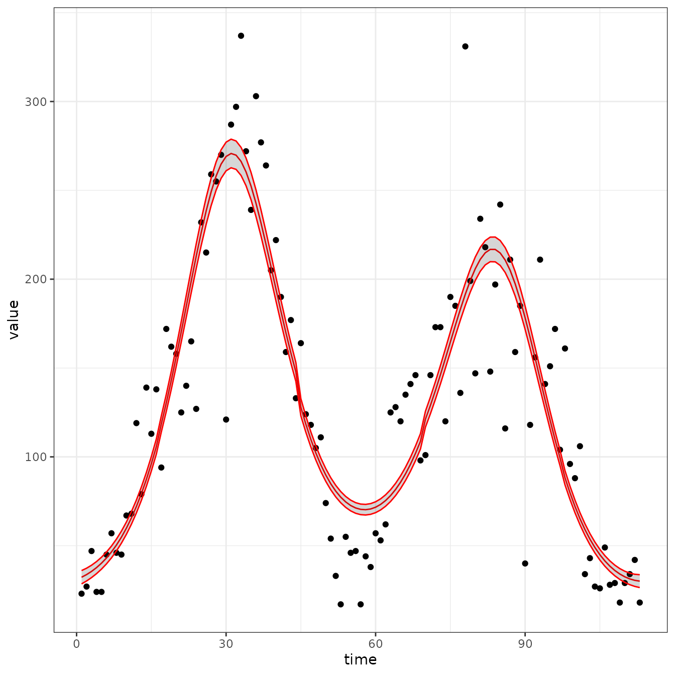

sir_cal = make_rbf_calibrator(dimension = 6)
mp_optimize(sir_cal)
#> Warning in (function (start, objective, gradient = NULL, hessian = NULL, :
#> NA/NaN function evaluation
#> Warning in (function (start, objective, gradient = NULL, hessian = NULL, :
#> NA/NaN function evaluation
#> Warning in (function (start, objective, gradient = NULL, hessian = NULL, :
#> NA/NaN function evaluation
#> Warning in (function (start, objective, gradient = NULL, hessian = NULL, :
#> NA/NaN function evaluation
#> Warning in (function (start, objective, gradient = NULL, hessian = NULL, :
#> NA/NaN function evaluation
#> $par
#>      params      params      params      params      params      params 
#>   0.1270159 128.1590763 128.3625346  -7.2152311   3.2483740  -3.8894784 
#>      params      params      params 
#>   0.4432874  -1.0387206  -2.2276442 
#> 
#> $objective
#> [1] 1029.754
#> 
#> $convergence
#> [1] 1
#> 
#> $iterations
#> [1] 103
#> 
#> $evaluations
#> function gradient 
#>      200      103 
#> 
#> $message
#> [1] "function evaluation limit reached without convergence (9)"

plot_fit(sir_cal)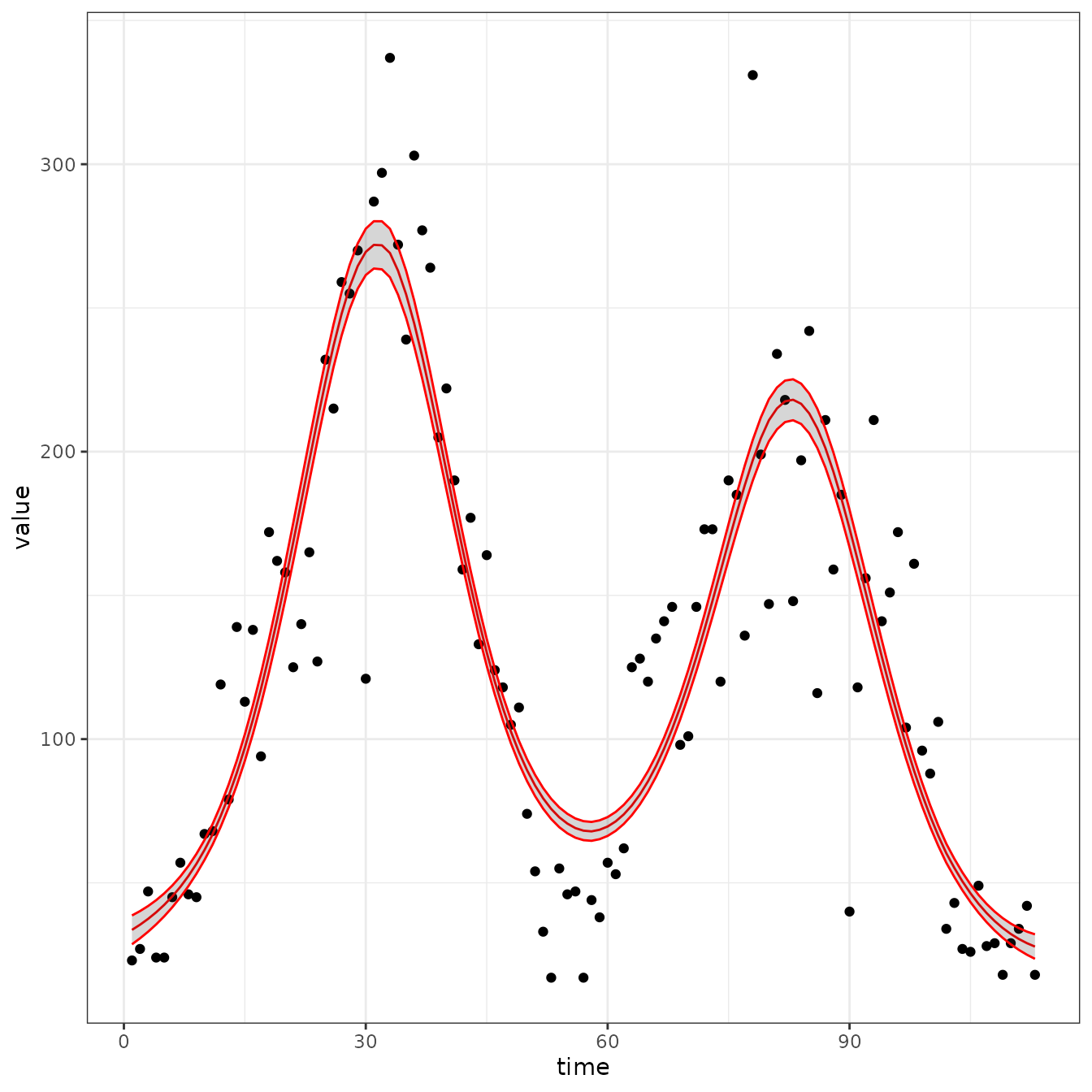

sir_cal = make_rbf_calibrator(dimension = 7)
mp_optimize(sir_cal)
#> Warning in (function (start, objective, gradient = NULL, hessian = NULL, :
#> NA/NaN function evaluation
#> Warning in (function (start, objective, gradient = NULL, hessian = NULL, :
#> NA/NaN function evaluation
#> Warning in (function (start, objective, gradient = NULL, hessian = NULL, :
#> NA/NaN function evaluation
#> Warning in (function (start, objective, gradient = NULL, hessian = NULL, :
#> NA/NaN function evaluation
#> Warning in (function (start, objective, gradient = NULL, hessian = NULL, :
#> NA/NaN function evaluation
#> Warning in (function (start, objective, gradient = NULL, hessian = NULL, :
#> NA/NaN function evaluation
#> Warning in (function (start, objective, gradient = NULL, hessian = NULL, :
#> NA/NaN function evaluation
#> Warning in (function (start, objective, gradient = NULL, hessian = NULL, :
#> NA/NaN function evaluation
#> Warning in (function (start, objective, gradient = NULL, hessian = NULL, :
#> NA/NaN function evaluation
#> Warning in (function (start, objective, gradient = NULL, hessian = NULL, :
#> NA/NaN function evaluation
#> Warning in (function (start, objective, gradient = NULL, hessian = NULL, :
#> NA/NaN function evaluation
#> Warning in (function (start, objective, gradient = NULL, hessian = NULL, :
#> NA/NaN function evaluation
#> Warning in (function (start, objective, gradient = NULL, hessian = NULL, :
#> NA/NaN function evaluation
#> Warning in (function (start, objective, gradient = NULL, hessian = NULL, :
#> NA/NaN function evaluation
#> Warning in (function (start, objective, gradient = NULL, hessian = NULL, :
#> NA/NaN function evaluation
#> $par
#>        params        params        params        params        params 
#>  1.971535e-02  7.543047e+03  4.314971e-03  3.005822e-01 -2.356461e+00 
#>        params        params        params        params        params 
#>  8.875691e-01 -4.221472e+00  8.522903e-01 -2.034926e+00  6.156743e-01 
#> 
#> $objective
#> [1] 951.6669
#> 
#> $convergence
#> [1] 0
#> 
#> $iterations
#> [1] 75
#> 
#> $evaluations
#> function gradient 
#>      160       76 
#> 
#> $message
#> [1] "relative convergence (4)"

plot_fit(sir_cal)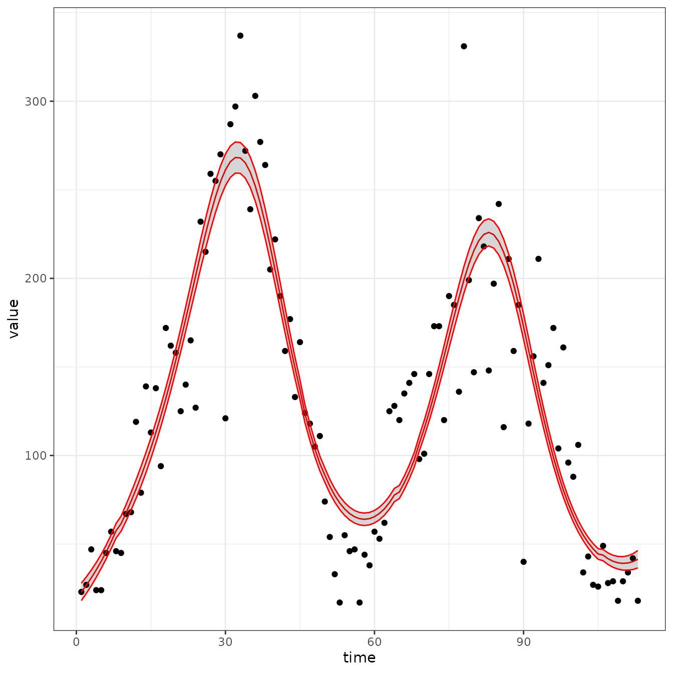

Interestingly we have now managed to fit gamma

mp_tmb_coef(sir_cal)
#>        term           mat row col      default  type      estimate    std.error
#> 1    params         gamma   0   0  0.100000000 fixed  1.971535e-02 6.841928e-03
#> 2  params.1             I   0   0  1.000000000 fixed  7.543047e+03 1.851632e+03
#> 3  params.2   report_prob   0   0  0.003333333 fixed  4.314971e-03 3.499032e-05
#> 4  params.3 time_var_beta   0   0 -0.006264538 fixed  3.005822e-01 1.627780e-01
#> 5  params.4 time_var_beta   1   0  0.001836433 fixed -2.356461e+00 1.402708e-01
#> 6  params.5 time_var_beta   2   0 -0.008356286 fixed  8.875691e-01 1.122606e-01
#> 7  params.6 time_var_beta   3   0  0.015952808 fixed -4.221472e+00 1.333442e-01
#> 8  params.7 time_var_beta   4   0  0.003295078 fixed  8.522903e-01 1.810992e-01
#> 9  params.8 time_var_beta   5   0 -0.008204684 fixed -2.034926e+00 1.118681e-01
#> 10 params.9 time_var_beta   6   0  0.004874291 fixed  6.156743e-01 2.701168e-01

This is a much slower recovery rate. Expected time in the R box is about one year! Not believeable, but the point is to make it easier to fit models so you can try more things.

mp_tmb_calibrator(
    spec = sf_sir
  , data = observed_data
  , traj = "reports"  
  , tv = mp_rbf("beta", dimension = 7)
  , par = c("gamma", "I", "report_prob")
  , outputs = c("reports", "beta")
)
#> ---------------------
#> Before the simulation loop (t = 0):
#> ---------------------
#> 1: S ~ N - I - R
#> 2: outputs_var_beta ~ group_sums(values_var_beta * time_var_beta[col_indexes_beta], row_indexes_beta, outputs_var_beta)
#> 
#> ---------------------
#> At every iteration of the simulation loop (t = 1 to T):
#> ---------------------
#> 1: beta ~ exp(outputs_var_beta[time_step(1)])
#> 2: infection ~ S * I * beta/N
#> 3: recovery ~ I * gamma
#> 4: S ~ S - infection
#> 5: I ~ I + infection - recovery
#> 6: R ~ R + recovery
#> 7: reports ~ infection * report_prob
#> 
#> ---------------------
#> After the simulation loop (t = T + 1):
#> ---------------------
#> 1: sim_reports ~ rbind_time(reports, obs_times_reports)
#> 
#> ---------------------
#> Objective function:
#> ---------------------
#> ~-sum(dpois(obs_reports, clamp(sim_reports)))

References

Elderd, Bret D., Vanja M. Dukic, and Greg Dwyer. 2006. “Uncertainty in Predictions of Disease Spread and Public Health Responses to Bioterrorism and Emerging Diseases.” Proceedings of the National Academy of Sciences 103 (42): 15693–97. https://doi.org/10.1073/pnas.0600816103.