Engine-Agnostic Model Specification Grammar

One of the main goals of macpan2 is to provide a flexible grammar for model specification that reduces friction when building upon and expanding an existing model. This goal complements the standard approach of modelling, which is to start simply and add complexity as needed.

There is a trade-off between the flexibility and the simplicity of the model grammar: specifying a simple model may not always be very concise, and there is a learning curve to the model grammar. However, it can be very powerful when it comes to specifying structured models, especially when they are cast as expansions of simple models. Such structured models can include:

multiple pathogen strains
multiple infection types (e.g., asymptomatic and symptomatic or mild and severe)
age-structure
multiple locations (a metapopulation model)
testing processes to identify infections
vaccination status

This vignette seeks to explain macpan2’s model specification grammar and in particular how one could take a simple model and expand it with additional structure.

Amuse bouche: a structured SIR model

A key to macpan2’s flexible model grammar is the use of functional forms to repeat the same kinds of calculations across model structures. For instance, consider an SIR model that has two pathogen strains (without co-infections):

Here,

$S$ , $I_x$ , and $R$ are the numbers of individuals that are susceptible, infected with strain $x$ ( $A$ or $B$ ), and recovered, respectively,
$N= S + I_A + I_B + R$ is the total population size,
$\beta_x$ is the transmission rate for strain $x$ ,
$\gamma$ is the recovery rate for infected individuals,¹
$\lambda_x = \beta_x (I_x)/N$ is the force of infection for strain $x$ .

We can cast this model as a system of difference equations, since this is how we will iterate them numerically in our simulation:

$\begin{align} S_{t+1} & = - [\beta_A (I_A)_t/N + \beta_B (I_B)_t/N] S_t, \\ (I_A)_{t+1} &= \phantom{-[} \beta_A (I_A)_t/N - \gamma (I_A)_t, \\ (I_B)_{t+1} &= \phantom{-[} \beta_B (I_B)_t/N - \gamma (I_B)_t, \\ R_{t+1} &= \phantom{-[} \gamma (I_A)_t + \gamma (I_B)_t. \end{align}$

Each force of infection, $\lambda_A = \beta_A (I_A)/N$ and $\lambda_B = \beta_B (I_B)/N$ has the same functional form, that is, using an expression like $\lambda = \beta I / N$ . When numerically simulating this model, it doesn’t take much effort to write out each calculation separately as something like:

lambda.A = beta.A * I.A / N
lambda.B = beta.B * I.B / N

However, in macpan2, we can specify a single functional form for it, for instance

lambda = beta * I / N

and then attach a ledger to the model object that tabulates specific instances of when this functional form is used to define a component of the model. In other words, this ledger should enumerate which specific subscripted lambda, beta, and I to use each time we invoke the associated functional form during the simulation.

In this case, there would only be two calculations in the force of infection ledger (one calculation per strain), but one can easily imagine a more complicated case. For instance, consider a relatively simple two-city age-structured metapopulation model with 10 age groups within each of two patches: there would be 10x10x2 = 200 force of infection terms of the same form (one per combination of age groups to capture the options for susceptible and infected interaction, repeated for each of the two patches).

Using functional forms and ledgers allows the modeller to focus on modelling questions, like the design of the model structure and the choice of expressions for the forces of infection, while macpan2 handles the bookkeeping, matching stratified variables with each other when calculating expressions. This approach cuts down on rote repetition when setting up model calculations, which in turn reduces the opportunity for bugs in the simulation code. It also means that expanding a model can be as simple as updating the calculation ledger, rather than error-prone editing of calculations in the simulation code.

While a modeller could write their own code to cut down on repetition when expanding a simple model (and many do), macpan2 provides a ready-made model specification grammar that enables easy model extension, especially when building product models, and that can readily interface with fast simulation and calibration engines, like TMB.

Appetizer: specifying the basic SIR model

Let’s start with specifying the basic SIR model, the foundation of the two-strain model above, in macpan2:

$\begin{align} S_{t+1} &= -\beta S_t I_t/N, \\ I_{t+1} &= \phantom{-} \beta S_t I_t/N - \gamma I_t, \\ R_{t+1} &= \phantom{-} \gamma I_t. \end{align}$

It will be helpful to set $\lambda = \beta I/N$ and recast the equations as:

$\begin{align} S_{t+1} &= -\lambda S_t, \\ I_{t+1} &= \phantom{-} \lambda S_t - \gamma I_t, \\ R_{t+1} &= \phantom{-} \gamma I_t. \end{align}$

Since the focus of this quickstart guide is macpan2’s model specification grammar, we have defined an SIR_starter() function to sweep some of the details of initializing a model object under the rug (for now, though we will revisit it later). All you need to know about SIR_starter() at this stage is that we will pass it some inputs to define the model using the model grammar and it will output a model object from which we can build a simulator. Our primary focus for the remainder of this vignette will be how the inputs to SIR_starter() are created.

The inputs to SIR_starter() are of two types:

index tables containing indices (labels) of model quantities,
ledgers that tabulate specific calculations required to simulate the model equations (based on the included functional forms).

The index tables we need to specify fall into two groups:

state: state names, $S$ , $I$ , and $R$ from the model equations
rate: rate names, $\beta$ , $\gamma$ , and the derived rate $\lambda$

We have identified two useful functional forms that we have baked into SIR_starter(). In this case, we’re thinking of these forms not necessarily as repeated calculations in this particular model, but as calculations that a modeller may want to repeat down the line, as they expand this simple model with additional structure (as we will do below). The forms are:

flow: Unsigned flows from one class to another of the form $rX$ , with $r>0$ being the per capita flow rate and $X$ being the occupancy of the state from which the flow originates. This calculation is repeated for all terms on the right-hand side of the recast system of difference equations above.
force of infection: The prevalence-dependent per capita rate of flow from susceptible classes to infectious classes of the form $\lambda = \beta I /N$ , used in calculating infection flows.

In this case, the flow form is repeated within these model equations, while the force of infection form is used only once. We’ve identified the force of infection as a functional form since we will want to repeat it later when expanding into the two-strain model. Either way, these forms are already baked into SIR_starter(), so our task will be creating a ledger for each of these forms to input into the function.

We start by creating the state and rate index tables:

## index tables to label model quantities -------------------------
state <- mp_index(Epi = c("S", "I", "R"))
rate <- mp_index(Epi = c("beta", "gamma", "lambda"))

The mp_index() function sets structures like data frames that tabulate the model quantity labels:

state

##  Epi
##    S
##    I
##    R

rate

##     Epi
##    beta
##   gamma
##  lambda

The Epi column name is unimportant in this simple model, but it will be key to stratifying model quantities with different features (such as epidemiological status, infection type, age group, location) in more complicated models.

For the flow form, we will create two ledgers: infection for the flow from $S$ to $I$ and recovery for the flow from $I$ to $R$ and then pass these as a list to the flow argument of SIR_starter(). We specify flows using the name of the state from which it originates (from_states), the state to which it goes (to_states), and a flow rate name (flow_rates).

We use the mp_join() function to create the infection ledger like so:

## infection ledger -------------------------
infection <- mp_join(
  from_states = mp_subset(state, Epi = "S"),
  to_states = mp_subset(state, Epi = "I"), 
  flow_rates = mp_subset(rate, Epi = "lambda")
)

The mp_join() function takes the options provided in each argument from_states, to_states, and flow_rates, e.g.

mp_subset(state, Epi = "S")

##  Epi
##    S

mp_subset(state, Epi = "I")

##  Epi
##    I

mp_subset(rate, Epi = "lambda")

##     Epi
##  lambda

and by default creates one entry in the ledger for each combination of these values (i.e., a full join). However, since there is only one value in each column, there is only one entry in the resulting ledger:

infection

##  from_states to_states flow_rates
##            S         I     lambda

The names of the arguments in the mp_join() function are tied to how the functional form baked into SIR_starter() is specified, but in general modellers can define their functional forms and the corresponding mp_join() argument names however they like.²

We create the recovery ledger in a similar way:

## recovery ledger -------------------------
recovery  <- mp_join(
  from_states = mp_subset(state, Epi = "I"),
  to_states = mp_subset(state, Epi = "R"),
  flow_rates = mp_subset(rate, Epi = "gamma")
)

recovery

##  from_states to_states flow_rates
##            I         R      gamma

Finally, the force_of_infection ledger is slightly different as it corresponds to a different functional form in SIR_starter() (so the mp_join() argument names are different):

## force of infection ledger -------------------------
# infection additionally involves the calculation of a force of infection
force_of_infection <- mp_join(
  infectious_states = mp_subset(state, Epi = "I"),
  transmission_rates = mp_subset(rate, Epi = "beta"),
  infection_flow_rates = mp_subset(rate, Epi = "lambda")
)

For this functional form, we need to specify the transmission_rates and infectious_states involved in computing the force of infection, as well as the names where we want to store the results of this calculation (infection_flow_rates) for use in the infection flow calculations.

Now we can use the SIR_starter() function to initialize our model object:

## SIR model object -------------------------
sir <- SIR_starter(
  # index tables
  state = state,
  rate = rate,
  # ledgers
  flow = list(
    infection,
    recovery
  ),
  force_of_infection = force_of_infection
)

We can create a model simulator using mp_dynamic_simulator()³, giving it the model object (model), initial values for each index (vectors), as well as the number of total time steps in the simulation (time_steps):

## SIR model simulator -------------------------
sir_simulator <- mp_dynamic_simulator(
  dynamic_model = sir,
  vectors = list(
    state = c(S = 999, I = 1, R = 0),
    rate = c(beta = 0.25, gamma = 0.1)
  ),
  time_steps = 100
)

Note that we’ve specified NA for lambda as it will be calculated for us using the force of infection functional form.

Then we can actually simulate the model by passing our model simulator to mp_trajectory():

## SIR model simulation results -------------------------
sir_results <- mp_trajectory(sir_simulator)

The output of the simulation is a long data frame:

head(sir_results)

##   matrix time    row col     value
## 1  state    1      S     998.75025
## 2  state    1      I       1.14975
## 3  state    1      R       0.10000
## 4   rate    1   beta       0.25000
## 5   rate    1  gamma       0.10000
## 6   rate    1 lambda       0.00025

The simulation output has several columns:

matrix: The matrix storing our values internally, corresponding to our two index tables, state and rate.
time: An internal time index, where time = 1 is the result after the first step through the simulation loop.
row: The primary label for the value (the row name in the corresponding matrix).
col: A secondary label for the value (the column name in the corresponding matrix). Since the outputs of this model (i.e. states and rates) are specified as vectors and not matrices, this column is empty for all entries. TODO: When would this be useful?
value: The numerical value.

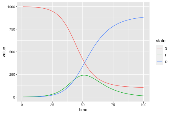
This output can be manipulated and plotted with standard tools, like dplyr and ggplot2, e.g.:

(sir_results
  |> filter(matrix == "state") # keep just the state variables at each point in time
  |> mutate(state = factor(row, levels = c("S", "I", "R"))) # to enforce logical state ordering in legend
  |> ggplot(aes(time, value, colour = state))
  +  geom_line()
)

(Above, we used the base R pipe operator, |>.)

If you prefer to make plots in base R, you can convert the long format data to wide format:

sir_results_wide <- (sir_results
    |> dplyr::filter(matrix == "state") # keep state variables at each point in time
    ## drop unneeded columns before pivoting
    |> dplyr::select(-c(matrix, col))
    |> tidyr::pivot_wider(id_cols = time, names_from = row)
)

head(sir_results_wide, n = 3)

## # A tibble: 3 × 4
##    time     S     I     R
##   <int> <dbl> <dbl> <dbl>
## 1     1  999.  1.15 0.1  
## 2     2  998.  1.32 0.215
## 3     3  998.  1.52 0.347

We can plot one state like so

with(sir_results_wide,
     plot(x = time,
          y = I,
          type = "l")
)

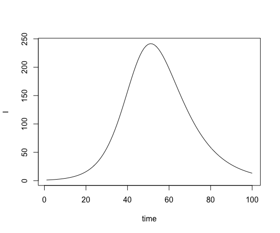
or multiple states on the same plot with

par(las = 1) ## horizontal y-axis ticks
matplot(sir_results_wide[, 1],
        sir_results_wide[,-1],
        type = "l",
        xlab = "time", ylab = "")
legend("left", col = 1:3, lty = 1:3, legend = state$labels())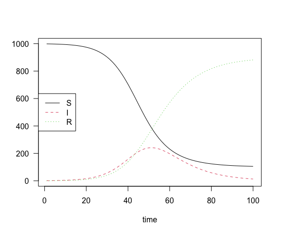

Main course: expanding the basic SIR with additional structure

As previously noted, we created a force of infection functional form ( $\beta I / N$ ) despite it only being used once to define the SIR model. However, if we consider the two-strain model from before, we see this calculation is repeated for each strain:

$\begin{align} \lambda_A &= \beta_A I_A/N \\ \lambda_B &= \beta_B I_B/N \end{align}$

Since we already have a form for the force of infection, we can easily expand our basic SIR with the strain-related structure to get the two-strain SIR model.

To define the two-strain model, we again must specify our state and rate index tables, as well as our infection, recovery, and force_of_infection ledgers.

We start by creating a new set of indices for the strains:

Strain_indices <- c("A", "B")

A simple approach would be to define a table of the new state and rate indices directly using the mp_index() function, as we did above:

state <- mp_index(
  Epi = c("S", rep("I", 2), "R"),
  Strain = c("", Strain_indices, "")
)

rate <- mp_index(
  Epi = c(rep(c("beta", "lambda"), 2), "gamma"),
  Strain = c(rep(c("A", "B"), each = 2), "")
)

However, this approach is less flexible if we want to build a complex model or if we already have a simpler, working model (like the SIR above) and want expand it with many strata and/or several different types of strata. We present an alternative approach below that is more verbose but far more flexible.

For the state, we want to cross $I$ with the different strains to create one $I$ compartment name per strain. We can do so using the mp_cartesian() function, which takes the Cartesian product of indices (all possible combinations across sets)⁴:

I_indices <- mp_cartesian(
  mp_subset(state, Epi = "I"),
  mp_index(Strain = Strain_indices)
)

I_indices

##  Epi Strain
##    I      A
##    I      B

This table stores all indices associated with the $I$ compartment.⁵

We then combine the newly-stratified $I$ indices with the other states that remain unchanged using the mp_union() function to make a state index table:

state <- mp_union(
  mp_subset(state, Epi = "S"),
  I_indices, 
  mp_subset(state, Epi = "R")
)

state

##  Epi Strain
##    S       
##    I      A
##    I      B
##    R

We update the rate index table similarly:

rate <- 
  mp_union(
  # stratify rates involved in the infection process by strain
  mp_cartesian(
    mp_subset(rate, Epi = c("beta", "lambda")),
    mp_index(Strain = Strain_indices)
  ),
  # recovery rate will be the same across strains
  mp_subset(rate, Epi = "gamma")
)

rate

##     Epi Strain
##    beta      A
##  lambda      A
##    beta      B
##  lambda      B
##   gamma

For the infection ledger, let’s see what our previous code for generating it yields now that we are (partially) stratifying by Strain:

# infection ledger from before
mp_join(
  from_states = mp_subset(state, Epi = "S"),
  to_states = mp_subset(state, Epi = "I"), 
  flow_rates = mp_subset(rate, Epi = "lambda")
)

##  from_states to_states flow_rates
##           S.       I.A   lambda.A
##           S.       I.B   lambda.A
##           S.       I.A   lambda.B
##           S.       I.B   lambda.B

As before, the default in mp_join() is to give all possible combinations for the indices (the full join), where the individual indices, denoted by values in the Epi and Strain columns, are dot-concatenated for the full quantity labels.

For this model, we want only two of these flows:

a flow between S and I.A with flow rate lambda.A
a flow between S and I.B with flow rate lambda.B

In other words, we want the Strain index on I to match with the Strain index on lambda. We can specify this within mp_join() when building the ledger like so:

## new infection ledger -------------------------
infection <- mp_join(
  from_states = mp_subset(state, Epi = "S"),
  to_states = mp_subset(state, Epi = "I"), 
  flow_rates = mp_subset(rate, Epi = "lambda"),
  by = list(
    to_states.flow_rates = "Strain"
  )
)

infection

##  from_states to_states flow_rates
##           S.       I.A   lambda.A
##           S.       I.B   lambda.B

Note the syntax of the by argument here. Each by list element will correspond to a pairwise join of two of the index tables passed to mp_join(). Which indices are involved in the join will correspond to the dot concatenated list element name (to_states.flow_rates), with the names coming from mp_join()’s argument names (to_states, flow_rates). The list element value should be a character string corresponding to the index table column name upon which to perform matches. In this case, the value is "Strain" because we want the “to state” labels and the “flow rate” labels to match based on the Strain index table column (I.A with lambda.A and I.B with lambda.B).

For the recovery ledger, we haven’t stratified gamma or R, so the default full join with the I labels yields exactly the flows we want:

recovery <- mp_join(
    from_states = mp_subset(state, Epi = "I"),
    to_states = mp_subset(state, Epi = "R"),
    flow_rates = mp_subset(rate, Epi = "gamma")
)
recovery

##  from_states to_states flow_rates
##          I.A        R.     gamma.
##          I.B        R.     gamma.

For the force of infection ledger, the full join yields many combinations that we don’t want:

mp_join(
  infection_flow_rates = mp_subset(rate, Epi = "lambda"),
  infectious_states = mp_subset(state, Epi = "I"),
  transmission_rates = mp_subset(rate, Epi = "beta")
)

##  infection_flow_rates infectious_states transmission_rates
##              lambda.A               I.A             beta.A
##              lambda.B               I.A             beta.A
##              lambda.A               I.B             beta.A
##              lambda.B               I.B             beta.A
##              lambda.A               I.A             beta.B
##              lambda.B               I.A             beta.B
##              lambda.A               I.B             beta.B
##              lambda.B               I.B             beta.B

We want the lambda, I, and beta labels all matched on the Strain column of the respective index tables. Internally, mp_join() performs pairwise joins, so we cannot specify a three-way by argument. Instead, we will specify two pairwise joins to the same effect:

## new force of infection ledger -------------------------
force_of_infection <- mp_join(
  infection_flow_rates = mp_subset(rate, Epi = "lambda"),
  infectious_states = mp_subset(state, Epi = "I"),
  transmission_rates = mp_subset(rate, Epi = "beta"),
  by = list(
    infection_flow_rates.infectious_states = "Strain", # first pairwise join
    infectious_states.transmission_rates = "Strain" # second pairwise join
  )
)

force_of_infection

##  infection_flow_rates infectious_states transmission_rates
##              lambda.A               I.A             beta.A
##              lambda.B               I.B             beta.B

Now we’re ready to build the two-strain model object and simulate it:

two_strain_model <- SIR_starter(
  # index tables
  state = state,
  rate = rate,
  # ledgers
  flow = list(
    infection,
    recovery
  ),
  force_of_infection = force_of_infection
)

two_strain_simulator <- mp_dynamic_simulator(
  dynamic_model = two_strain_model,
  vectors = list(
    state = c(S = 998, I.A = 1, I.B = 1, R = 0),
    rate = c(beta.A = 0.25, gamma = 0.1, beta.B = 0.2)
  ),
  time_steps = 100
)

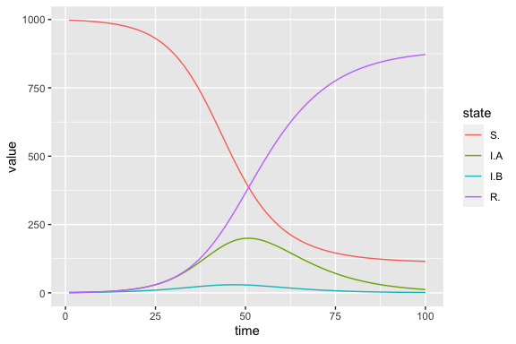
two_strain_results <- (mp_trajectory(two_strain_simulator)
  |> filter(matrix == "state")                    
)

levels <- unique(two_strain_results$row) # get state variables in the desired order

(two_strain_results # keep state variables at each point in time
  |> mutate(state = factor(row, levels = levels)) # to enforce logical state ordering in plot
  |> ggplot(aes(time, value, colour = state))
  +  geom_line()
)

Dessert: understanding model simulation in `macpan2`

As mentioned, we’ve hidden some of the details of initializing a model object within the SIR_starter() function:

## helper function to simplify the exposition in this vigette -----------
SIR_starter <- function(
  # index tables for model quantities
  state,
  rate,
  # ledgers tabulating the use of different functional forms
  flow, # list of individual ledgers
  force_of_infection
){
  
  ## Set up expressions list for each functional form --------------
  ## names refer to when the calculation gets performed relative to 
  ## the simulation time-step loop (before, during, ...)
  ## FIXME: we should not be referring to a specific engine in
  ## a vignette about an 'engine-agnostic grammar'
  expr_list <- mp_tmb_expr_list(
    before = list(
      ## aggregations
        N ~ sum(state)
    ),
    during = list(
      ## force of infections
        rate[infection_flow_rates] ~
          state[infectious_states] * rate[transmission_rates] / N
  
      ## unsigned individual flows
      , flow_per_time ~ state[from_states] * rate[flow_rates]
  
      ## state update
      , total_inflow ~ group_sums(flow_per_time, to_states, state)
      , total_outflow ~ group_sums(flow_per_time, from_states, state)
      , state ~ state + total_inflow - total_outflow
    )
  )
  
  ## Ledgers for each specific calculation --------------
  ledgers <- list(
    flow = mp_ledgers(flow),
    force_of_infection = mp_ledgers(force_of_infection)
  )
  
  ## Initialize vectors from index tables (with all zeros for values) --------------
  # used as placeholders for user input
  init_vecs <- list(
    state = mp_structured_vector(state),
    rate = mp_structured_vector(rate)
  )
  
  ## Initialize model object -----------------
  mp_dynamic_model(
    expr_list = expr_list,
    ledgers = ledgers,
    init_vecs = init_vecs
  )
}

This function definition shows how all the pieces fit together. The expressions list expr_list is perhaps the most interesting as it contains all of the functional forms used to simulate the model, including some we explored above (unsigned flows, force of infection), as well as some that we didn’t discuss (total inflow, total outflow, state update). The ledgers and init_vecs are just set up to ensure that the ledgers and initial conditions for simulation get attached to the model object correctly.

These topics will be discussed fully in a future vignette.

Amuse bouche: a structured SIR model

Appetizer: specifying the basic SIR model

Main course: expanding the basic SIR with additional structure

Dessert: understanding model simulation in macpan2

Dessert: understanding model simulation in `macpan2`