Hello World
This vignette shows how to simulate from the SI model, which is I think is the simplest possible model of epidemiological transmission. Here is the code for defining an SI model (see this short article on how to find other example models).
library(ggplot2)
library(dplyr)
library(tidyr)
library(macpan2)
si = mp_tmb_model_spec(
    before = S ~ N - I
  , during = mp_per_capita_flow(
        from      = "S"            # compartment from which individuals flow
      , to        = "I"            # compartment to which individuals flow
      , rate      = "beta * I / N" # expression giving per-capita flow rate
      , flow_name = "infection"    # name of absolute flow rate = beta * I * S/N
    )
  , default = list(N = 100, I = 1, beta = 0.25)
)
print(si)
## ---------------------
## Default values:
## quantity value
## N 100.00
## I 1.00
## beta 0.25
## ---------------------
##
## ---------------------
## Before the simulation loop (t = 0):
## ---------------------
## 1: S ~ N - I
##
## ---------------------
## At every iteration of the simulation loop (t = 1 to T):
## ---------------------
## 1: mp_per_capita_flow(from = "S", to = "I", rate = "beta * I / N",
## flow_name = "infection")Simulating from this model requires choosing the number of time-steps
to run and the model outputs to generate. Syntax for simulating
macpan2 models is designed to combine with standard data
prep and plotting tools in R, as we demonstrate with the following
code.
library(ggplot2)
library(dplyr)
si_plot = (si

 ## macpan2
 |> mp_simulator(
        time_steps = 50
      , outputs = c("I", "infection")
    )
 |> mp_trajectory()

 ## dplyr
 |> mutate(quantity = case_match(matrix
      , "I" ~ "Prevalence"
      , "infection" ~ "Incidence"
    ))

 ## ggplot2
 |> ggplot()
 + geom_line(aes(time, value))
 + facet_wrap(~ quantity, scales = "free")
 + theme_bw()
)
## Warning: There was 1 warning in `mutate()`.
## ℹ In argument: `quantity = case_match(matrix, "I" ~ "Prevalence", "infection" ~
## "Incidence")`.
## Caused by warning:
## ! `case_match()` was deprecated in dplyr 1.2.0.
## ℹ Please use `recode_values()` instead.
print(si_plot)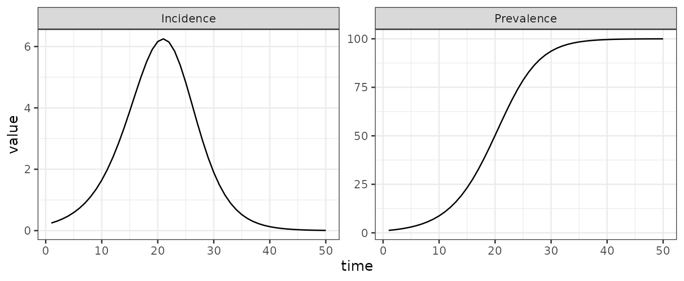
(Above, we used the base
R pipe operator, |>.)
The remainder of this article looks at each step required to create this plot in more detail, and discusses alternative approaches.
Creating a Simulator
The first step is to produce a simulator object, which can be used to
generate simulation results. This object can be produced using the
mp_simulator function, which takes the following
arguments.
-
model: A model specification object, such assi. -
time_steps: How many time steps should the epidemic simulator run for? -
outputs: The model variables to return in simulation output. Functionsmp_state_vars()andmp_flow_vars()can be used to programmatically output all state or flow variables respectively. -
default(optional) : Allows one to update the default parameter values and initial conditions provided in the model specification (see the argumentdefaultabove in themp_tmb_model_specfunction). Any variables that are not specified indefaultwill be left at the values in the specification.
si_simulator = mp_simulator(
    model = si
  , time_steps = 50
  , outputs = c("I", "infection")
)
si_simulator
## ---------------------
## Before the simulation loop (t = 0):
## ---------------------
## 1: S ~ N - I
##
## ---------------------
## At every iteration of the simulation loop (t = 1 to 50):
## ---------------------
## 1: infection ~ S * (beta * I/N)
## 2: S ~ S - infection
## 3: I ~ I + infectionThis si_simulator object contains all of the information
required to generate model simulations of I and
infection over 50 time steps, without actually generating
the simulations. This more interesting step of simulation is covered in
the next section. But before
moving on we explain why we separate the step of creating a simulator
from the step of running simulations.
The reason for two steps is to optimize performance in more computationally challenging applications of the software than those covered in this article. The step of creating the simulator object is more computationally intensive than the next step of actually generating the simulations. Therefore this separation is useful when a single simulator can be used to repeatedly generate many different simulations. Three common examples requiring repeated simulations from the same simulator are:
- for models with stochasticity so that the output is different for each run,
- for calibrating model parameters to data using iterative optimization tools,
- and for running different scenarios by updating certain parameters before simulation.
Because macpan2 is primarily developed for such
computationally challenging iterative simulation problems, we believe
that it is better to introduce these two steps as distinct from the very
beginning. Although two steps might seem unnecessarily complex within
the context of this article, keeping them separate will make life easier
when working with more realistic workflows and models.
Generating Simulations
Now that we have a simulation engine object,
si_simulator, we use it to generate simulation results
using the mp_trajectory() function. The results come out in
long (or
“narrow”) format, where there is exactly one value per row:
si_results = mp_trajectory(si_simulator)
si_results |> head(8)
## matrix time row col value
## 1 I 1 0 0 1.2475000
## 2 infection 1 0 0 0.2475000
## 3 I 2 0 0 1.5554844
## 4 infection 2 0 0 0.3079844
## 5 I 3 0 0 1.9383066
## 6 infection 3 0 0 0.3828223
## 7 I 4 0 0 2.4134907
## 8 infection 4 0 0 0.4751841The simulation results are output as a data frame with the following columns:
-
matrix: Which matrix does a value come from? All variables are represented as matrices, although in this article we only consider 1-by-1 matrices. -
time: The time index from1totime_steps. -
row,col: Placeholders for variable components in more complicated structured models (not covered in this article, but useful for example when S and I in different age groups or geographic locations are tracked separately). -
value: The simulated value for a particular state and time step.
(Note that the row and col placeholders can
be completely omitted by using
options(macpan2_collapse_traj = TRUE) near the top of your
script that calls mp_trajectory())
Processing Results
macpan2 does not provide any data manipulation or
plotting tools (although there are a few in
macpan2helpers). The philosophy is to focus on the engine
and modelling interface, but to provide outputs in formats that are easy
to use with other data processing packages, like ggplot2,
dplyr, and tidyr, all of which readily make
use of data in long format.
In the graphs above for example, we required a step that renames the model variables into something that makes more sense for the graphical presentation. Here we reproduce this, but take a little more care to produce a tidier dataset.
si_results = (si_results
  |> mutate(matrix = case_match(matrix
      , "I" ~ "Prevalence"
      , "infection" ~ "Incidence"
    ))
  |> rename(quantity = matrix)
  |> select(time, quantity, value)
)
print(head(si_results, 8L))
## time quantity value
## 1 1 Prevalence 1.2475000
## 2 1 Incidence 0.2475000
## 3 2 Prevalence 1.5554844
## 4 2 Incidence 0.3079844
## 5 3 Prevalence 1.9383066
## 6 3 Incidence 0.3828223
## 7 4 Prevalence 2.4134907
## 8 4 Incidence 0.4751841Here we rename the I state variable as the disease
prevalence (number of currently infected individuals). Because this is a
discrete-time model, we can reinterpret the infection as
the incidence (number of newly infected individuals) over one time step.
Note that this approach to calculating incidence only works if the time
period over which incidence is measured corresponds to the length of one
time step. If this assumption is not met – for example if the time step
is one day but incidence data are reported every week – then other
approaches to computing incidence that are not covered here must be
taken.
We can generate a ggplot from this dataset as we did
above. If you want to use base R plots, you can convert the long format
data to wide format using the tidyr package.
library(tidyr)
si_results_wide <- (si_results
  |> tidyr::pivot_wider(
      , id_cols = time
      , names_from = quantity
    )
  |> rename(Time = time)
)
head(si_results_wide, n = 3)
## # A tibble: 3 × 3
## Time Prevalence Incidence
## <int> <dbl> <dbl>
## 1 1 1.25 0.248
## 2 2 1.56 0.308
## 3 3 1.94 0.383
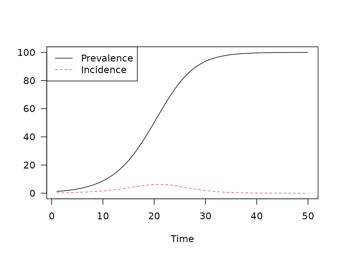
or
par(las = 1) ## horizontal y-axis ticks
matplot(
    si_results_wide[, 1]
  , si_results_wide[,-1]
  , type = "l"
  , xlab = "Time", ylab = ""
)
legend("topleft"
  , col = 1:3
  , lty = 1:3
  , legend = c("Prevalence", "Incidence")
)