Quickstart Guide, part 2: specifying and simulating a structured compartmental model • macpan2

library(macpan2)
#> Warning in checkMatrixPackageVersion(): Package version inconsistency detected.
#> TMB was built with Matrix version 1.6.1.1
#> Current Matrix version is 1.5.4.1
#> Please re-install 'TMB' from source using install.packages('TMB', type = 'source') or ask CRAN for a binary version of 'TMB' matching CRAN's 'Matrix' package
library(dplyr)
#> 
#> Attaching package: 'dplyr'
#> The following object is masked from 'package:macpan2':
#> 
#>     all_equal
#> The following objects are masked from 'package:stats':
#> 
#>     filter, lag
#> The following objects are masked from 'package:base':
#> 
#>     intersect, setdiff, setequal, union
library(ggplot2)
library(tidyr)

This article is the counterpart to vignette('quickstart', package = 'macpan2'), but instead of explaining the spec and sim of a simple SIR, we describe the new components introduced by trying to specify a product model. While the new “productify” functionality should make most of the content of this article obsolete eventually, this article can serve as a resource for users until then.

SIR Vaccination model

A good place to start with product models is the sir_vax starter model which stratifies a standard SIR model to include vaccination status.

print(sir_vax_dir <- system.file("starter_models", "sir_vax", package = "macpan2"))
#> [1] "/home/runner/work/_temp/Library/macpan2/starter_models/sir_vax"

As in the case of a simple SIR model the population is divided into compartments for susceptible, infected, and recovered individuals. However the population is also divided into compartments for vaccinated and unvaccinated individuals. So where a simple SIR model has three compartments the SIR_vax model has six. This is reflected in the variables.csv file in the model directory which now has two columns.

#> Epi       ,Vax
#> S         ,unvax
#> I         ,unvax
#> R         ,unvax
#> N         ,unvax
#> sigma     ,unvax
#> beta      ,unvax
#> foi       ,unvax
#> infection ,unvax
#> gamma     ,unvax
#> S         ,vax
#> I         ,vax
#> R         ,vax
#> N         ,vax
#> sigma     ,vax
#> beta      ,vax
#> foi       ,vax
#> infection ,vax
#> gamma     ,vax
#> foi       ,
#>           ,vax_rate

The row of the file specifies the name of each column; so the first column is called Epi and the second column is called Vax. predictably the Epi column lists compartment and parameter names relevant to epidemiological status and the Vax column similarly relates to vaccination status. Some parameters (e.g. gamma) which in an SIR model have a single value now have two values to reflect the differences in behavior in vaccinated and unvaxxinated people. Other parameters (e.g. vax_rate) have only a single value (in this case because only susceptible people will be vaccinated). Epi parameters that vary based on vax status will have the parameter name repeated in the Epi column but will have differing status labels in the Vax column. When referring to specific compartments or parameters we concatenate their labels in each column with a ., so the compartment for the unvaccinated susceptible population is called S.unvax. If a variable has no label in a given column then that entry is left blank but the concatonation dot is still included (so vax_rate is properly referred to as .vax_rate).

Flows in product models are specified by the flows.csv file in the model definition directory.

#> from    ,to    ,flow      ,type       ,from_partition ,to_partition ,flow_partition ,from_to_partition ,from_flow_partition ,to_flow_partition
#> S       ,I     ,infection ,per_capita ,Epi            ,Epi          ,Epi            ,Vax               ,Vax                 ,Null
#> I       ,R     ,gamma     ,per_capita ,Epi            ,Epi          ,Epi            ,Vax               ,Vax                 ,Null
#> S.unvax ,S.vax ,vax_rate  ,per_capita ,Epi.Vax        ,Epi.Vax      ,Vax            ,                  ,                    ,Null

Notice that the three right most columns, which unused in single stratum models now have an important role. In particular they are there to ensure that compartments of one stratum flow into other compartments of the same stratum. Without them the S.vax compartment would have flows both to I.vax and I.unvax. There are three such columns from_to_partition, from_flow_partition and to_flow_partition, in general two of these columns should have entries and the third should be blank or have the null_partition label specified in settings.json. The from_to_partition column indicates which partitions should be used to math from and to compartments. In the example the flow from S to I indicates the Vax partition should be used so S.vax flows to I.vax and S.unvax to I.unvax. The from_flow_partition column indicates which partition should be used to match from compartments with flow variables. In this example the flow from I to R has Vax in the from_flow_partition so the flow from I.unvax to R.unvax is matched with the gamma.unvax variable. In principle the to_flow_partition column can be used to match flow parameters to flow via their to compartment rather than their from compartment however in this example we have used the other two columns so the to_flow_column has a Null entry. Notice that the flow from S.unvax to S.vax is different from the other flows because there are no corresponding flows from I.unvax to I.vax or from R.unvax to R.vax. In this case the from_partition and the to_partition are both Epi.Vax because the from and to compartments are specified using both partitions, the flow_partition is specified as Vax because the rate of vaccination is governed by the .dose_rate variable which has no entry in the Epi partition. There is no need to use the final three columns since the compartments involved in the flow are given explicitly rather than as a group as was the case for the other flows.

#> [
#>   {
#>     "group_partition" : "Vax",
#>     "group_names" : ["unvax", "vax"],
#>     "output_partition" : "Epi.Vax",
#>     "output_names" : ["N.unvax", "N.vax"],
#>     "simulation_phase" : "during_pre_update",
#>     "input_partition" : "Epi",
#>     "arguments" : ["S", "I", "R"],
#>     "expression" : "sum(S, I, R)"
#>   },
#>   {
#>     "group_partition" : "Vax",
#>     "group_names" : ["unvax", "vax"],
#>     "output_partition" : "Epi.Vax", 
#>     "output_names" : ["foi.unvax", "foi.vax"],
#>     "simulation_phase" : "during_pre_update",
#>     "input_partition" : "Epi",
#>     "arguments" : ["I", "beta", "N"],
#>     "expression" : "I * beta / clamp(N)" 
#>   },
#>   {
#>     "filter_partition" : "Epi",
#>     "filter_names" : ["foi"],
#>     "output_partition" : "Epi.Vax",
#>     "output_names" : ["foi."],
#>     "simulation_phase" : "during_pre_update",
#>     "input_partition" : "Vax",
#>     "arguments" : ["unvax", "vax"],
#>     "expression" : "unvax + vax"
#>   },
#>   {
#>     "filter_partition" : "Epi.Vax",
#>     "filter_names" : ["foi.", "sigma.unvax", "sigma.vax", "infection.unvax", "infection.vax"],
#>     "group_partition" : "Vax",
#>     "group_names" : ["unvax", "vax"],
#>     "output_partition" : "Epi.Vax",
#>     "output_names" : ["infection.unvax", "infection.vax"],
#>     "simulation_phase" : "during_pre_update",
#>     "input_partition" : "Epi",
#>     "arguments" : ["foi", "sigma"],
#>     "expression" : "foi * sigma"
#>   }
#> ]

The derivations.json file from the model definition directory largely the same as it would be for single stratum models. On key distinction is that now each derivation can correspond to multiple different equations, this is reflected in the existence of multiple entries in the group_names as well as output_names fields. If we take the first derivation in the above file as an example we can see that the expression being evaluated is sum(S, I, R). The group_names field has entries unvax and vax (the group_partition field defines which partition the group_names are related to). The output_names field also has two entries N.unvax and N.vax which are the names of the variables this derivation will compute values for. Taken together we see that this single derivation produces two distinct equations, N.unvax = sum(I.unvax, S.unvax, R.unvax) and N.vax = sum(S.vax, I.vax, R.vax).

#> {
#>   "required_partitions" : ["Epi", "Vax"],
#>   "null_partition" : "Null",
#>   "state_variables" : ["S.unvax", "I.unvax", "R.unvax", "S.vax", "I.vax", "R.vax"],
#>   "flow_variables" : ["infection.unvax", "infection.vax", "gamma.unvax", "gamma.vax", ".vax_rate"]
#> }

The only notable difference between the settings.json files for single stratum and multi-strata models is that multi-strata models will have multiple required_partitions. It’s also worth noting that the null_partition entry defines what should be entered in whichever of the from_to_partition, from_flow_partition and to_from_partition isn’t being used in the flows.csv file.

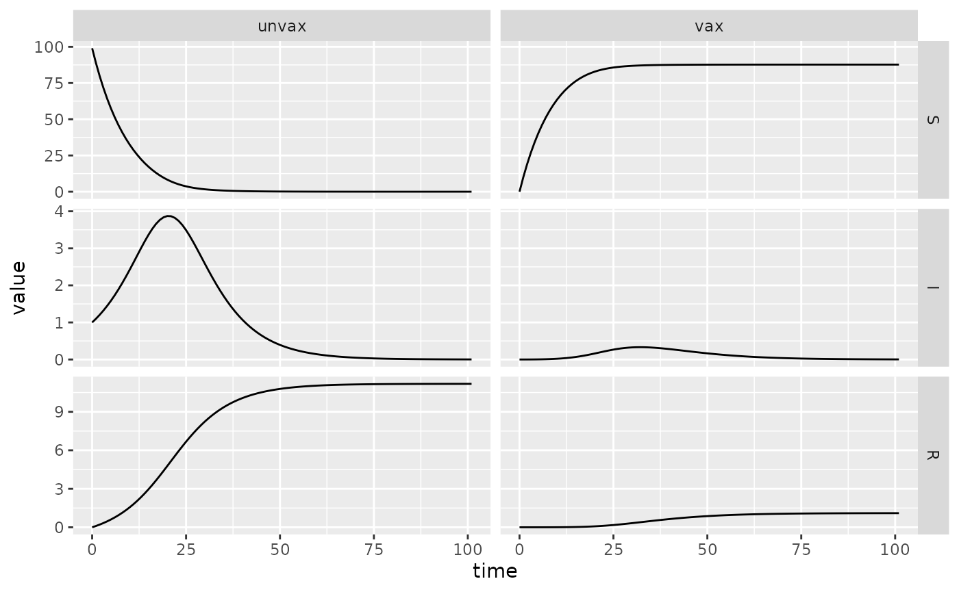
sir_vax = Compartmental(sir_vax_dir)
## TODO: add this 'facet grid' functionality to macpan2helpers::visCompartmental
draw_vis(sir_vax, x_mult = 200, y_mult = 100)

sir_vax_sim = sir_vax$simulators$tmb(time_steps = 100L
  , state = c(S.unvax = 99, I.unvax = 1, R.unvax = 0, S.vax = 0, I.vax = 0, R.vax = 0)
  , flow = c(
        infection.unvax = 0, infection.vax = 0
      , gamma.unvax = 0.1, gamma.vax = 0.1
      , .vax_rate = 0.1
    )
  , sigma.unvax = 1
  , sigma.vax = 0.01
  , beta.unvax = 0.2
  , beta.vax = 0.2
  , foi.unvax = empty_matrix
  , foi.vax = empty_matrix
  , foi. = empty_matrix
  , N.unvax = empty_matrix
  , N.vax = empty_matrix
)

(sir_vax_sim$report() 
 %>% separate_wider_delim("row", ".", names = c("Epi", "Vax"))
 %>% mutate(Epi = factor(Epi, levels = c("S", "I", "R")))
 %>% ggplot()
 + facet_grid(Epi~Vax, scales = "free")
 + geom_line(aes(time, value))
)