ODE Solvers, Process Error, and Difference Equations
Source:vignettes/state_updaters.Rmd
state_updaters.RmdThe McMasterPandemic project has focused on using
discrete time difference equations to solve the dynamical system. Here
we describe experimental features that allow one to update the data
differently. In particular, it is now possible to use a Runge-Kutta 4
ODE solver (to approximate the solution to the continuous time analogue)
as well as the Euler Multinomial distribution to generate process error.
These features have in principle been available for most of the life of
macpan2, but only recently have they been given a more
convenient interface.
In order to use this interface, models must be rewritten using
explicit declarations of state updates. By explicitly declaring what
expressions correspond to state updates, macpan2 is able to
modify the method of updating without further user input. This makes it
easier to compare difference equations (i.e. Euler steps), ODEs
(i.e. Runge-Kutta), and process error (i.e. Euler Multinomial) runs for
the same underlying dynamical model.
To declare a state update one replaces formulas in the
during argument of a model spec to include calls to the
mp_per_capita_flow() function. As an example we will modify
the SI model to include explicit state updates. The original form of the
model looks like this.
library(macpan2)
si_implicit = mp_tmb_model_spec(
    before = list(S ~ N - I)
  , during = list(
        infection ~ beta * S * I / N
      , S ~ S - infection
      , I ~ I + infection
    )
  , default = list(I = 1, N = 100, beta = 0.25)
)
print(si_implicit)
#> ---------------------
#> Default values:
#>  quantity  value
#>         I   1.00
#>         N 100.00
#>      beta   0.25
#> ---------------------
#>
#> ---------------------
#> Before the simulation loop (t = 0):
#> ---------------------
#> 1: S ~ N - I
#>
#> ---------------------
#> At every iteration of the simulation loop (t = 1 to T):
#> ---------------------
#> 1: infection ~ beta * S * I/N
#> 2: S ~ S - infection
#> 3: I ~ I + infection
The modified version looks like this.
si_explicit = mp_tmb_model_spec(
    before = list(S ~ N - I)
  , during = list(mp_per_capita_flow("S", "I", infection ~ beta * I / N))
  , default = list(I = 1, N = 100, beta = 0.25)
)
print(si_explicit)
#> ---------------------
#> Default values:
#>  quantity  value
#>         I   1.00
#>         N 100.00
#>      beta   0.25
#> ---------------------
#>
#> ---------------------
#> Before the simulation loop (t = 0):
#> ---------------------
#> 1: S ~ N - I
#>
#> ---------------------
#> At every iteration of the simulation loop (t = 1 to T):
#> ---------------------
#> 1: mp_per_capita_flow(from = "S", to = "I", rate = infection ~ beta *
#>      I/N)
With this explicit spec we can make three different simulators.
si_euler = (si_explicit
  |> mp_euler()
  |> mp_simulator(time_steps = 50, outputs = "infection")
)
si_rk4 = (si_explicit
  |> mp_rk4()
  |> mp_simulator(time_steps = 50, outputs = "infection")
)
si_euler_multinomial = (si_explicit
  |> mp_euler_multinomial()
  |> mp_simulator(time_steps = 50, outputs = "infection")
)
library(dplyr)
#>
#> Attaching package: 'dplyr'
#> The following object is masked from 'package:macpan2':
#>
#>     all_equal
#> The following objects are masked from 'package:stats':
#>
#>     filter, lag
#> The following objects are masked from 'package:base':
#>
#>     intersect, setdiff, setequal, union
trajectory_comparison = list(
    euler = mp_trajectory(si_euler)
  , rk4 = mp_trajectory(si_rk4)
  , euler_multinomial = mp_trajectory(si_euler_multinomial)
) |> bind_rows(.id = "update_method")
print(head(trajectory_comparison))
#>   update_method    matrix time row col     value
#> 1         euler infection    1   0   0 0.2475000
#> 2         euler infection    2   0   0 0.3079844
#> 3         euler infection    3   0   0 0.3828223
#> 4         euler infection    4   0   0 0.4751841
#> 5         euler infection    5   0   0 0.5888103
#> 6         euler infection    6   0   0 0.7280407
library(ggplot2)
(trajectory_comparison
  |> rename(`Time Step` = time, Incidence = value)
  |> ggplot()
  + geom_line(aes(`Time Step`, Incidence, colour = update_method))
)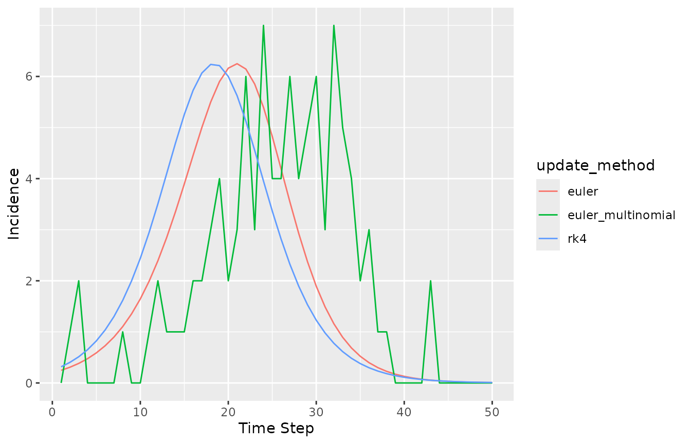
The incidence trajectory is different for the three update methods, even though the initial values of the state variables were identical in all three cases.
mp_initial(si_euler)
#>   matrix row col  value
#> 1      N         100.00
#> 2      I           1.00
#> 3   beta           0.25
#> 4      S          99.00
mp_initial(si_euler_multinomial)
#>   matrix row col  value
#> 1      N         100.00
#> 2      I           1.00
#> 3   beta           0.25
#> 4      S          99.00
mp_initial(si_rk4)
#>   matrix row col  value
#> 1      N         100.00
#> 2      I           1.00
#> 3   beta           0.25
#> 4      S          99.00
The incidence is different, even during the first time step, because each state update method causes different numbers of susceptible individuals to become infectious at each time step. Further, incidence here is defined for a single time step and so this number of new infectious individuals is exactly the incidence.
Branching Flows and Process Error
 siv = mp_tmb_model_spec(
    before = list(S ~ N - I - V)
  , during = list(
        mp_per_capita_flow("S", "I", infection ~ beta * I / N)
      , mp_per_capita_flow("S", "V", vaccination ~ rho)
    )
  , default = list(I = 1, V = 0, N = 100, beta = 0.25, rho = 0.1)
)
print(siv)
#> ---------------------
#> Default values:
#>  quantity  value
#>         I   1.00
#>         V   0.00
#>         N 100.00
#>      beta   0.25
#>       rho   0.10
#> ---------------------
#>
#> ---------------------
#> Before the simulation loop (t = 0):
#> ---------------------
#> 1: S ~ N - I - V
#>
#> ---------------------
#> At every iteration of the simulation loop (t = 1 to T):
#> ---------------------
#> 1: mp_per_capita_flow(from = "S", to = "I", rate = infection ~ beta *
#>      I/N)
#> 2: mp_per_capita_flow(from = "S", to = "V", rate = vaccination ~
#>      rho)
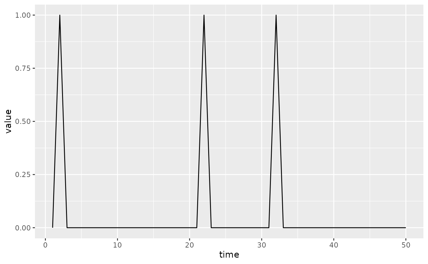
(siv
 |> mp_euler_multinomial()
 |> mp_simulator(50, "infection")
 |> mp_trajectory()
 |> ggplot()
  + geom_line(aes(time, value))
)
Internal Design
sir = mp_tmb_model_spec(
  during = list(
      N ~ S + I + R
    , mp_per_capita_flow("S", "I", "beta * I / N", "infection")
    , mp_per_capita_flow("I", "R", "(1 - p) * gamma", "recovery")
    , mp_per_capita_flow("I", "D", "p * gamma", "death")
  )
)
ChangeComponent() classes
Model specs contain a set of three lists: * before :
instructions to run before the simulation loop begins. *
during : instructions to run at each iteration of the
simulation loop. * after : instructions to run after the
simulation loop ends.
The simplest way to define these lists is using two-sided R formulas.
But in the during list one may specify different types of
list components, which are of class ChangeComponent.
Internally, standard R formulas are converted into an object of class
Formula, which is the simplest kind of
ChangeComponent. Another important
ChangeComponent is the PerCapitaFlow type,
which is used for standard flows from one compartment to another.
The list of change components, which is just the during
field but ensuring that all elements are valid
ChangeComponent objects, can be obtained using the
change_components() method in a model spec object.
cc = sir$change_components()
print(cc)
#> [[1]]
#> N ~ S + I + R
#>
#> [[2]]
#> From: S
#> To: I
#> Per-capita rate expression: beta * I/N
#> Absolute rate symbol: infection
#> [[3]]
#> From: I
#> To: R
#> Per-capita rate expression: (1 - p) * gamma
#> Absolute rate symbol: recovery
#> [[4]]
#> From: I
#> To: D
#> Per-capita rate expression: p * gamma
#> Absolute rate symbol: death
All ChangeComponent objects must have the following
methods.
The change_frame() method
Returns a data frame with two columns: * state : state
variable being changed (i.e. updated at each step) * change
: signed absolute flow rates (variables or expressions that don’t
involve any state variables)
An example of this data frame for a flow from S to
I is as follows.
cc[[2]]$change_frame()
#>   state     change
#> 1     S -infection
#> 2     I +infection
For a simple Formula change component this data frame is
just an empty two-column data frame with zero rows.
cc[[1]]$change_frame()
#> [1] state  change
#> <0 rows> (or 0-length row.names)
The flow_frame() method
Returns a data frame with three columns. * size :
variable (often a state variable or function of state variables) that
gives the size of the population being drawn from in a flow (e.g. S is
the size of an infection flow). * change : unsigned
absolute flow rates. * rate : per-capita flow rates
(variables or expresions that sometimes involve state variables).
An example of this data frame for a flow from S to
I is as follows.
cc[[2]]$flow_frame()
#>   size    change       rate         abs_rate
#> 1    S infection beta * I/N S * (beta * I/N)
For a simple Formula change component this data frame is
just an empty three-column data frame with zero rows.
cc[[1]]$flow_frame()
#> [1] size     change   rate     abs_rate
#> <0 rows> (or 0-length row.names)
ChangeModel() classes
The ChangeModel objects combine the information in lists
of ChangeComponent objects, so that they specify a full
model. It expands the concept of before,
during, and after into a more refined set of
steps. All of these methods return lists of two-sided formulas.
-
before_loop(): Thebeforelist formulas. -
once_start(): Formulas to evaluate at the start of theduringlist, and which will not be repeated (or modified and repeated) throughout expansions of theduringloop. An example of such an expansion is a Runge-Kutta differential equation solver that reuses expressions in an iterative manner. Formulas returned byonce_during()are useful for specifying exogeneous changes (e.g., time-varying parameters) that occur once per time-step but that should not change throughout the within-time-step iterations of a differential equation solver. -
before_flows(): Formulas to evaluate before the absolute flow rates are computed. -
update_flows(): Formulas that update the flows, usingflow_frame()methods of individualChangeComponentobjects. -
before_state(): Formulas to evaluate before the state vector is updated. -
update_state(): Formulas that update the state vector, usingchange_frame()method s of individualChangeComponentobjects. -
after_state(): Formulas to evaluate after the state vector is updated. -
once_end(): Formulas to evaluate at the end of theduringlist, and which will not be repeated throughout (similar toonce_start()). -
after_loop(): Theafterlist formulas.
The ChangeModel objects also have
flow_frame() and change_frame() methods for
combining the outputs of these methods within the individual
ChangeComponent objects. An example for an SIR model gives
the flow_frame() and change_frame() output as
follows.
state   change
-----   ------
S       -infection
I       +infection
I       -recovery
R       +recovery
size change rate
---- ------ ----
S infection beta * I / N
I recovery gammaThe update_flows() method The
update_state() method makes use of this
flow_frame() to produce the
si = mp_tmb_library("starter_models", "sir", package = "macpan2")
si$change_model
#> Classes 'SimpleChangeModel', 'ChangeModelDefaults', 'ChangeModel', 'Base' <environment: 0x55e43cf9d8c8>
#> after_loop : function ()
#> after_state : function ()
#> all_user_aware_names : function ()
#> before_flows : function ()
#> before_loop : function ()
#> before_state : function ()
#> change_classes : function ()
#> change_frame : function ()
#> check : function ()
#> duplicated_change_names : function ()
#> flow_frame : function ()
#> no_change_components : function ()
#> once_finish : function ()
#> once_start : function ()
#> other_generated_formulas : function ()
#> update_flows : function ()
#> update_state : function ()
#> user_formulas : function ()
si$change_model$flow_frame()
#>   size    change       rate         abs_rate
#> 1    S infection beta * I/N S * (beta * I/N)
#> 2    I  recovery      gamma      I * (gamma)
si$change_model$change_frame()
#>   state     change
#> 1     S -infection
#> 2     I +infection
#> 3     I  -recovery
#> 4     R  +recovery
si$change_model$update_state()
#> [[1]]
#> S ~ -infection
#> <environment: 0x55e43d423980>
#>
#> [[2]]
#> I ~ +infection - recovery
#> <environment: 0x55e43d423980>
#>
#> [[3]]
#> R ~ +recovery
#> <environment: 0x55e43d423980>
si$change_model$update_flows()
#> $S
#> $S[[1]]
#> infection ~ beta * I/N
#> <environment: 0x55e43d4d7f60>
#>
#>
#> $I
#> $I[[1]]
#> recovery ~ gamma
#> <environment: 0x55e43d4d7f60>
spec = mp_tmb_model_spec(
  during = list(
      mp_per_capita_flow("A", "B", "a", "r")
    , mp_per_capita_flow("B", "C", "b", "rr")
  )
)
spec$change_model$update_flows()
#> $A
#> $A[[1]]
#> r ~ a
#> <environment: 0x55e43d952e00>
#>
#>
#> $B
#> $B[[1]]
#> rr ~ b
#> <environment: 0x55e43d952e00>
UpdateMethod() classes
In order to define a state updater one must define a new
UpdateMethod class. These classes are required to update
three methods that do not take any arguments: before,
during, and after. Each of these methods are
required to return a list of two-sided formulas giving the expression
list for the three phases of the simulation: before the simulation loop,
at every iteration of the simulation loop, and after the simulation
loop. Examples of UpdateMethod classes include:
EulerUpdateMethod, RK4UpdateMethod,
EulerMultinomialUpdateMethod, and
HazardUpdateMethod.
The constructors of these UpdateMethod classes often
have a field of class ChangeModel, which specifies how to
sort the components of
Relationship to Ordinary Differential Equation Solvers
It is instructive to view these state update methods as approximate solutions to ordinary differential equations (ODEs). We consider ODEs of the following form.
Where the per-capita rate of flowing from compartment to compartment is , and is the number of individuals in the th compartment. We allow each to depend on any number of state variables and time-varying parameters. For example, for an SIR model we have (for readability we use ). In this case , , and all other values of are zero. Here the force of infection, , depends on a state variable .
Although each state-update method presented below can be thought of as an approximate solution to this ODE, they can also be thought of as dynamical models in their own right. For example, the Euler-multinomial model is a useful model of process error.
Euler
The simplest approach is to just pretend that the ODEs are difference equations. In this case, at each time-step, each state variable is updated as follows. The SIR example is as follows.
Euler-Multinomial
The Euler-multinomial state update method assumes that the number of individuals that move from one box to another in a single time-step is a random non-negative integer, coming from a particular multinomial distribution that we now describe.
The probability of staying in the th box through an entire time-step is assumed to be the following (TODO: relate this to Poisson processes).
This probability assumes that the are held constant throughout the entire time-step, although they can change when each time-step begins.
The probability of moving from box to box in one time-step is given by the following.
This probability is just the probability of not staying in box , which is , and specifically going to box , which is assumed to be given by this expression .
Let be the random number of individuals that move from box to box in one time-step. The expected value of is . However, these random variables are not independent events, because the total number of individuals, , has to remain constant through a single time-step (at least in the models that we are currently considering).
To account for this non-independence, we collect the associated with a from compartment into a vector . We collect similar vector of probabilities, . Each is a random draw from a multinomial distribution with trials and probability vector, .
Once these random draws have been made, the state variables can be updated at each time-step as follows.
Note that we do not actually need to generate values for the diagonal elements, , because they cancel out in this update equation. We also can ignore any such that .
Under the SIR example we have a particularly simple Euler-binomial distribution because there are no branching flows – when individuals leave S they can only go to I and when they leave I they can only go to R. These two flows are given by the following distributions.
In models with branching flows we would have multinomial distributions. But in this model the state update is given by the following equations.
Hazard
The Hazard update-method uses the expected values associated with the Euler-multinomial described above. In particular, the state variables are updated as follows.
The SIR model would be as follows.
More explicitly for the compartment this would be.
Linearizing at Each Time-Step
Because the could depend on any state variable, the ODE above is generally non-linear. However, we could linearize the model at every time-step and explicitly compute the matrix exponential to find the approximate state update.
Hazard in models including more than unbalanced per-capita flows
The perfectly balanced per-capita flows approach used above does not always work. For example, virus shedding to a wastewater compartment does not involve infected individuals flowing into a wastewater compartment, because people do not become wastewater obviously. In such models we need to think more clearly about how to use the Hazard approximation.
For such cases we can modify the differential equation to include an arbitrary number of absolute inflows and outflows.
Where is the absolute rate at which increases due to mechanism and is the absolute rate at which decreases due to mechanism .