Structured SI Model with Kronecker Products in macpan2 • macpan2

Introduction

This document illustrates how to implement structured compartmental models in macpan2 using Kronecker products to define state vectors, parameter matrices, and flows over stratified dimensions. As an example, we stratify an SI model along the following dimensions: age group, vaccination status, and symptom severity.

model_dimensions = c("age", "vax", "symp")
age = c("young", "old")
vax = c("unvax", "vax")
symp = c("mild", "severe")

Utilities and Packages

We load the necessary packages and define some utility functions that simplify the construction of named vectors and matrices over these stratification dimensions.

library(macpan2)
library(ggplot2)
library(tidyr)
library(dplyr)
library(stringr)

We overwrite the base R Kronecker product operator, %x%, to consistently preserve row and column names. This operator will be used often when defining model structure. It returns the same numerical results as base R, but with consistently named rows and columns.

`%x%` <- mp_kronecker_operator(`*`)

The ones_vec() utility creates a named vector of ones over the cross-product of the input character vectors (strata). It uses Kronecker products to ensure the names follow the same ordering convention as Kronecker-structured vectors and matrices elsewhere in the model.

ones_vec = function(...) {
  nms = list(...)
  vecs = lapply(nms, \(x) setNames(rep(1, length(x)), x))
  Reduce(`%x%`, vecs)
}

The diagonal() utility is much like the base-R diag() function, but takes its row and column names from the names of the input vector.

diagonal = function(x) {
    if (is.matrix(x)) 
      stop("can only produce a square diagonal matrix for a vector")
    if (length(x) == 1) return(x)
    nms = names(x)
    x = diag(x)
    dimnames(x) = list(nms, nms)
    return(x)
}

The identity() function takes character vectors and returns an identity matrix over their Cartesian product. It uses ones_vec() and diagonal() to define the dimension names and place ones on the diagonal.

identity = function(...) ones_vec(...) |> diagonal()

The ones_col() (ones_row()) function takes character vectors and returns a column (row) vector of ones, with row (column) names based on the Cartesian product of the input strata.

ones_col = function(...) ones_vec(...) |> t() |> t()
ones_row = function(...) ones_col(...) |> t()

Here are a few examples.

identity(age, vax)

##             young.unvax young.vax old.unvax old.vax
## young.unvax           1         0         0       0
## young.vax             0         1         0       0
## old.unvax             0         0         1       0
## old.vax               0         0         0       1

ones_col(age, vax, symp)

##                    [,1]
## young.unvax.mild      1
## young.unvax.severe    1
## young.vax.mild        1
## young.vax.severe      1
## old.unvax.mild        1
## old.unvax.severe      1
## old.vax.mild          1
## old.vax.severe        1

ones_row(vax)

##      unvax vax
## [1,]     1   1

The ones_col(), ones_row(), and identity() functions make it easier to build vectors and matrices that align with stratified model dimensions, enabling clear and consistent operations like summing over strata or selecting specific blocks.

Initial State Vectors

We now use Kronecker products to initialize the state vectors S (susceptible) and I (infectious) over the stratification dimensions.

S = c(young = 75, old = 25) %x% c(unvax = 1, vax = 0)
I = c(young = 1, old = 0) %x% c(unvax = 1, vax = 0) %x% c(mild = 1, severe = 0)
print(S)

## young.unvax   young.vax   old.unvax     old.vax 
##          75           0          25           0

print(I)

##   young.unvax.mild young.unvax.severe     young.vax.mild   young.vax.severe 
##                  1                  0                  0                  0 
##     old.unvax.mild   old.unvax.severe       old.vax.mild     old.vax.severe 
##                  0                  0                  0                  0

Model Parameters

We define default values for the following parameters:

Baseline transmission
Vaccination rates
Vaccine efficacy
Contact matrix
Symptom severity probabilities
Multiplicative effects of stratification on susceptibility and infectivity.

beta = 0.4
contact_matrix = rbind(
  young = c(young = 0.8, old = 0.2),
  old   = c(young = 0.2, old = 0.8)
)
symp_probs = rbind(mild = 0.6, severe = 0.4)
susceptibility_age = rbind(young = 0.9, old = 1)
infectivity_age = cbind(young = 1, old = 0.9)
infectivity_vax = cbind(unvax = 1, vax = 0.8)
infectivity_symp = cbind(mild = 0.95, severe = 1)
vax_rates = rbind(young = 0.1, old = 0.4)
VE = rbind(unvax = 0, vax = 0.8)

Note that instead of c for constructing vectors, we use rbind (for column vectors) and cbind (for row vectors). It is good practice to be explicit about the orientation of vectors when Kronecker products are involved.

Derived State Vectors

To define flows and compute quantities like force of infection or vaccination rates, we often need to aggregate or restrict the original state vectors by strata. Derived state vectors let us isolate relevant subpopulations or repeat totals to match dimensional structure in downstream operations.

M_unvax = identity(age) %x% cbind(unvax = 1, vax = 0)
M_S = identity(age) %x% ones_row(vax)
M_I = identity(age) %x% ones_row(vax, symp)
M_N = ones_col(vax, symp)
S_unvax = M_unvax %*% S
N_age = (M_S %*% S) + (M_I %*% I)
N = N_age %x% M_N
print(S_unvax)

##       [,1]
## young   75
## old     25

print(N_age)

##       [,1]
## young   76
## old     25

print(N)

##   young.unvax.mild young.unvax.severe     young.vax.mild   young.vax.severe 
##                 76                 76                 76                 76 
##     old.unvax.mild   old.unvax.severe       old.vax.mild     old.vax.severe 
##                 25                 25                 25                 25

Note that N repeats the total population size within each age group to match the structure of the force of infection. S_unvax isolates the unvaccinated susceptible compartments, which are the only ones eligible for vaccination flows.

Per-Capita Transmission Matrix

We construct the full per-capita transmission matrix by combining component matrices using Kronecker products and elementwise multiplication.

B_age = (
    beta 
  * contact_matrix 
  * (susceptibility_age %x% infectivity_age)
)
B_vax = (1 - VE) %x% infectivity_vax
B_symp = infectivity_symp
B = B_age %x% B_vax %x% B_symp
print(B_age)

##       young    old
## young 0.288 0.0648
## old   0.080 0.2880

print(B_vax)

##       unvax  vax
## unvax   1.0 0.80
## vax     0.2 0.16

print(B_symp)

##      mild severe
## [1,] 0.95      1

print(B)

##             young.unvax.mild young.unvax.severe young.vax.mild young.vax.severe
## young.unvax          0.27360             0.2880       0.218880          0.23040
## young.vax            0.05472             0.0576       0.043776          0.04608
## old.unvax            0.07600             0.0800       0.060800          0.06400
## old.vax              0.01520             0.0160       0.012160          0.01280
##             old.unvax.mild old.unvax.severe old.vax.mild old.vax.severe
## young.unvax       0.061560          0.06480    0.0492480       0.051840
## young.vax         0.012312          0.01296    0.0098496       0.010368
## old.unvax         0.273600          0.28800    0.2188800       0.230400
## old.vax           0.054720          0.05760    0.0437760       0.046080

The per-capita transmission matrix maps infectious compartments to susceptible compartments and determines the force of infection associated with each susceptible stratum. The row names give the susceptible strata, and the column names the infectious strata.

Per-Capita Force of Infection

The force of infection is computed by multiplying the per-capita transmission matrix by the normalized infectious population.

foi = B %*% (I / N)
print(foi)

##                [,1]
## young.unvax 0.00360
## young.vax   0.00072
## old.unvax   0.00100
## old.vax     0.00020

Absolute Flows

We compute total flows due to infection and vaccination by multiplying per-capita rates by the relevant state vectors.

infection = foi * S
vaccination = vax_rates * S_unvax
print(infection)

##              [,1]
## young.unvax 0.270
## young.vax   0.000
## old.unvax   0.025
## old.vax     0.000

print(vaccination)

##       [,1]
## young  7.5
## old   10.0

Allocation Matrices

In structured models, flows often act on families of compartments rather than individual compartments. This can obscure which specific sub-compartments are gaining or losing individuals. Allocation matrices resolve this by mapping flow vectors into change vectors that align with the structure of state vectors.

They allow us to:

Distribute outflows from a compartment to multiple destination compartments (e.g., infections split by symptom severity).
Apply signed changes within a state vector (e.g., moving individuals from unvaccinated to vaccinated compartments within the susceptible state vector).

This ensures that each flow is properly aligned with the compartments it affects.

A_infection = identity(age, vax) %x% symp_probs
A_vaccination = identity(age) %x% rbind(unvax = -1, vax = 1)
infection_S = infection
infection_I = A_infection %*% infection
vaccination_S = A_vaccination %*% vaccination
print(infection_S)

##              [,1]
## young.unvax 0.270
## young.vax   0.000
## old.unvax   0.025
## old.vax     0.000

print(infection_I)

##                     [,1]
## young.unvax.mild   0.162
## young.unvax.severe 0.108
## young.vax.mild     0.000
## young.vax.severe   0.000
## old.unvax.mild     0.015
## old.unvax.severe   0.010
## old.vax.mild       0.000
## old.vax.severe     0.000

print(vaccination_S)

##              [,1]
## young.unvax  -7.5
## young.vax     7.5
## old.unvax   -10.0
## old.vax      10.0

Euler Step Update

Using the change vectors produced using products of allocation matrices and state vectors, we update the original state vectors with a forward Euler step.

S_new = S - infection_S + vaccination_S
I_new = I + infection_I
print(S_new)

##               [,1]
## young.unvax 67.230
## young.vax    7.500
## old.unvax   14.975
## old.vax     10.000

print(I_new)

##                     [,1]
## young.unvax.mild   1.162
## young.unvax.severe 0.108
## young.vax.mild     0.000
## young.vax.severe   0.000
## old.unvax.mild     0.015
## old.unvax.severe   0.010
## old.vax.mild       0.000
## old.vax.severe     0.000

Model Specification

We formalize the model specification with mp_tmb_model_spec, defining the derived quantities, flows, and update rules.

spec = mp_tmb_model_spec(
  before = list(
      B_age ~ (
          beta 
        * contact_matrix 
        * (susceptibility_age %x% infectivity_age)
      )
    , B_vax ~ (1 - VE) %x% infectivity_vax
    , B_symp ~ infectivity_symp
    , B ~ B_age %x% B_vax %x% B_symp

  ),
  during = list(
    
    # derived state vectors
      N_age ~ (M_S %*% S) + (M_I %*% I)
    , N ~ N_age %x% M_N
    , S_unvax ~ M_unvax %*% S
    
    # state-dependent per-capita rates
    , foi ~ B %*% (I / N)
    
    # absolute flow vectors
    , infection ~ foi * S
    , vaccination ~ vax_rates * S_unvax
    
    # absolute change vectors
    , infection_S ~ -infection
    , infection_I ~ A_infection %*% infection
    , vaccination_S ~ A_vaccination %*% vaccination
    
    # state update (euler step)
    , S ~ S + infection_S + vaccination_S
    , I ~ I + infection_I
  ),
  
  # initial state vectors
  inits = nlist(S, I),
  
  default = nlist(
    # parameter scalars
      beta
  
    # parameter vectors
    , vax_rates, VE
    , susceptibility_age
    , infectivity_age, infectivity_vax, infectivity_symp
    
    # parameter matrices
    , contact_matrix
    
    # state vector transformation matrices
    , M_S, M_I, M_N, M_unvax
    
    # allocation matrices
    , A_infection, A_vaccination
    
    # absolute flow and change vectors
    #   - included here so that row names can be used 
    #     in simulated trajectories
    #   - if removed from this list, the simulations
    #     will use generic integer IDs for each 
    #     stratum
    , infection, vaccination
    , infection_S, infection_I, vaccination_S
  )
)

Simulation and Plots

We simulate the model over time and visualize the resulting trajectories of the state vectors and flow rates by stratification. The first step is to generate the simulations.

## state vectors
state = c("S", "I")

## absolute flow rates
flow = c("infection", "vaccination")

# absolute change vectors
change = c("infection_S", "infection_I", "vaccination_S")

traj = (spec 
  |> mp_simulator(time_steps = 100, outputs = c(state, flow, change))
  |> mp_trajectory() 
  
  ## separate row names into 
  ## names for each stratum
  |> separate_wider_delim(row
      , delim = "."
      , names = model_dimensions
      , too_few = "align_start"
  )
  
  ## make stratum names easier to read
  |> mutate(vax = case_when(
        vax == "unvax" ~ "Unvaccinated"
      , vax == "vax" ~ "Vaccinated"
  ))
  |> mutate(age = str_to_title(age))
) 

print(traj)

## # A tibble: 3,400 × 7
##    matrix       time age   vax          symp  col    value
##    <chr>       <int> <chr> <chr>        <chr> <chr>  <dbl>
##  1 infection       1 Young Unvaccinated NA    ""     0.27 
##  2 infection       1 Young Vaccinated   NA    ""     0    
##  3 infection       1 Old   Unvaccinated NA    ""     0.025
##  4 infection       1 Old   Vaccinated   NA    ""     0    
##  5 vaccination     1 Young NA           NA    ""     7.5  
##  6 vaccination     1 Old   NA           NA    ""    10    
##  7 infection_S     1 Young Unvaccinated NA    ""    -0.27 
##  8 infection_S     1 Young Vaccinated   NA    ""     0    
##  9 infection_S     1 Old   Unvaccinated NA    ""    -0.025
## 10 infection_S     1 Old   Vaccinated   NA    ""     0    
## # ℹ 3,390 more rows

Here is a plot of the state vector trajectories.

(traj
  |> filter(matrix %in% state) 
 
  ## make names easier to read
  |> mutate(state = case_when(
        matrix == "S" ~ "Susceptible"
      , matrix == "I" ~ "Infectious"
  ))
  |> mutate(state = if_else(
        state == "Infectious"
      , sprintf("%s\n(%s)", state, symp)
      , state
  ))
  
  ## plot
  |> ggplot() 
  + aes(time, value) 
  + geom_line() 
  + facet_grid(state ~ age + vax, space = 'free', scales = 'free') 
  + scale_x_continuous(breaks = c(0, 40, 80))
  + theme_bw()
)

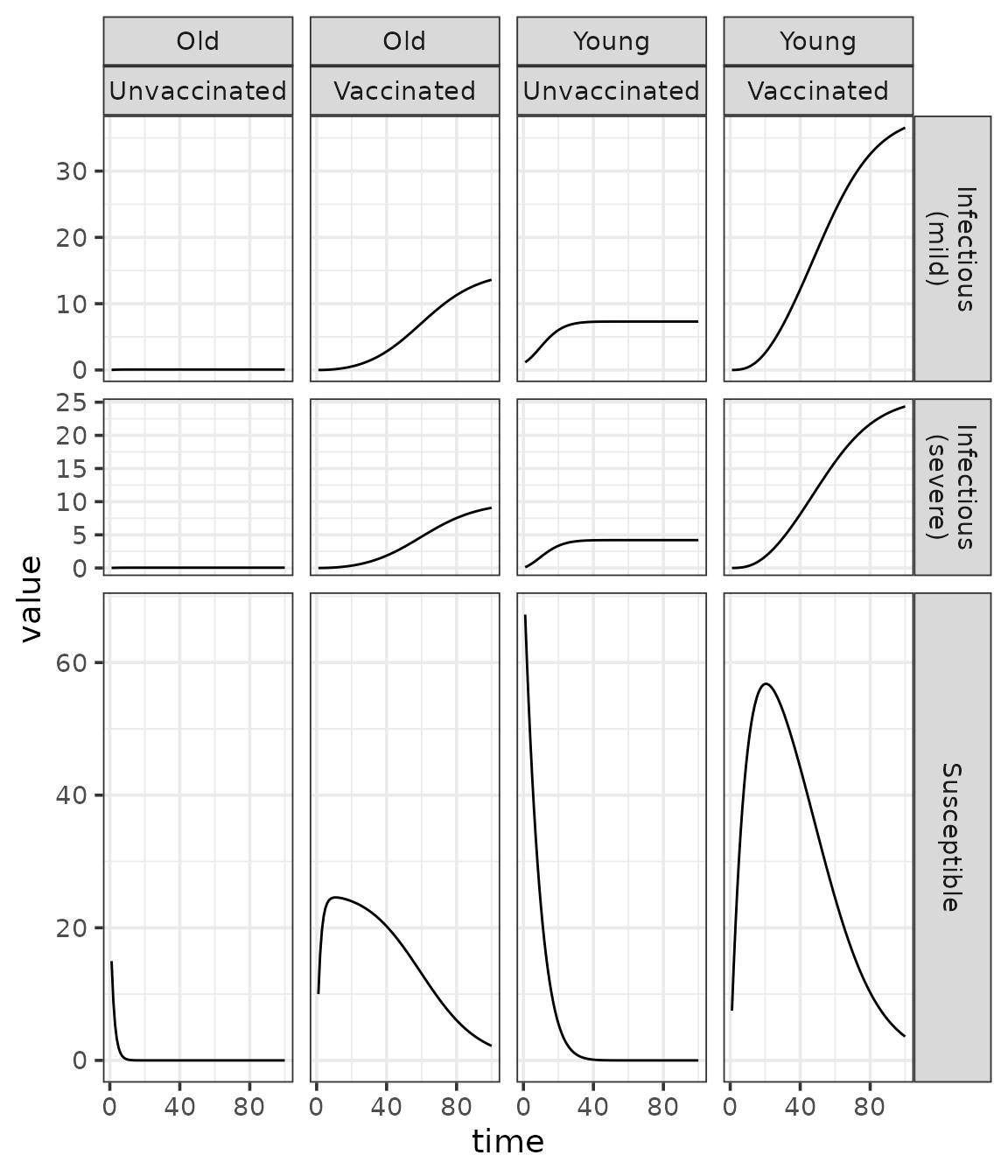
Structured SI models have the potential to become more interesting relative to the unstructured version. For a simple example in the above plot, two susceptible compartments display intermediate peaks that reflect a balance between vaccination and infection processes. In contrast, the susceptible compartment in the unstructured SI model can only decrease over time. You could produce this plot for different values of the parameters (e.g., vaccine efficacy) to explore how these differences affect dynamics.

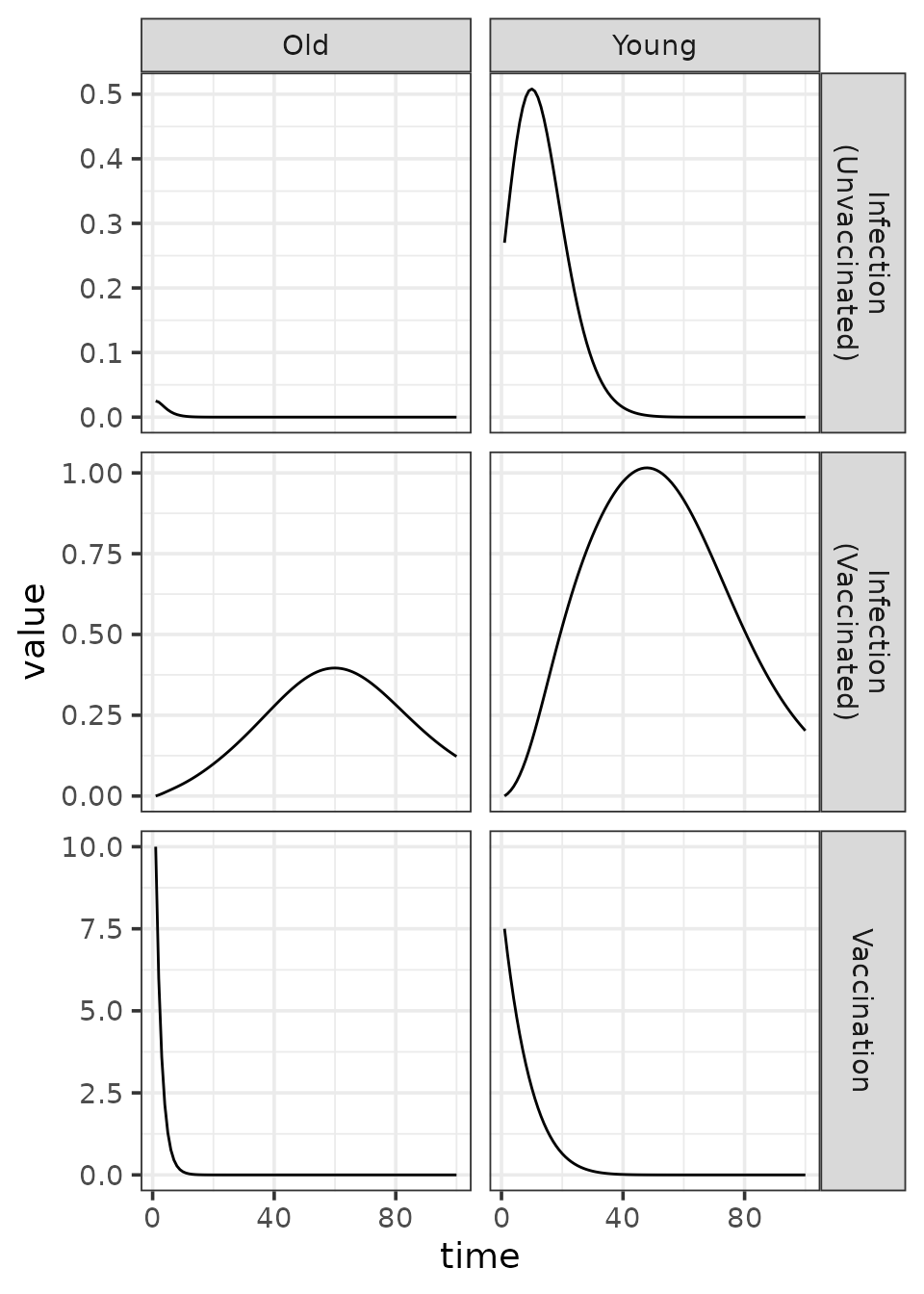
We can make a similar plot of the absolute rates of flow (per time step) among compartments. These flow rates are stored in the infection and vaccination vectors.

(traj
  |> filter(matrix %in% flow)
  
  |> mutate(matrix = str_to_title(matrix))
  |> mutate(flow = if_else(
        matrix == "Infection"
      , sprintf("%s\n(%s)", matrix, vax)
      , matrix
  ))
 
  |> ggplot() 
  + aes(time, value) 
  + geom_line() 
  + facet_grid(flow ~ age, scales = 'free')
  + scale_x_continuous(breaks = c(0, 40, 80))
  + theme_bw()
)

In structured models, absolute flow rates translate into process-specific rates of change of state variables in a more complex way than in unstructured models. One example of this added complexity is that flows alone do not determine how individuals are distributed across symptom status compartments. To address this, allocation matrices – A_infection and A_vaccination – are used to map each process-specific flow onto the appropriate rate of change in the state variables. These matrices define how the flows are distributed across strata, such as symptom status. The plot below illustrates the resulting changes in the state vector.

(traj
  |> filter(matrix %in% change)
  
  |> separate_wider_delim(matrix
      , delim = "_"
      , names = c("flow", "state")
  )
  |> mutate(state = case_when(
        state == "S" ~ "Susceptible"
      , state == "I" ~ "Infectious"
  ))
  |> mutate(state = if_else(
        state == "Infectious"
      , sprintf("%s\n(%s)", state, symp)
      , state
  ))
  |> mutate(flow = sprintf("Change due to\n%s", flow))
 
  |> ggplot() 
  + aes(time, value, colour = vax) 
  + geom_line() 
  + facet_grid(flow + state ~ age, scales = 'free')
  + scale_x_continuous(breaks = c(0, 40, 80))
  + theme_bw()
  + guides(colour = guide_legend(position = "bottom", title = ""))
)

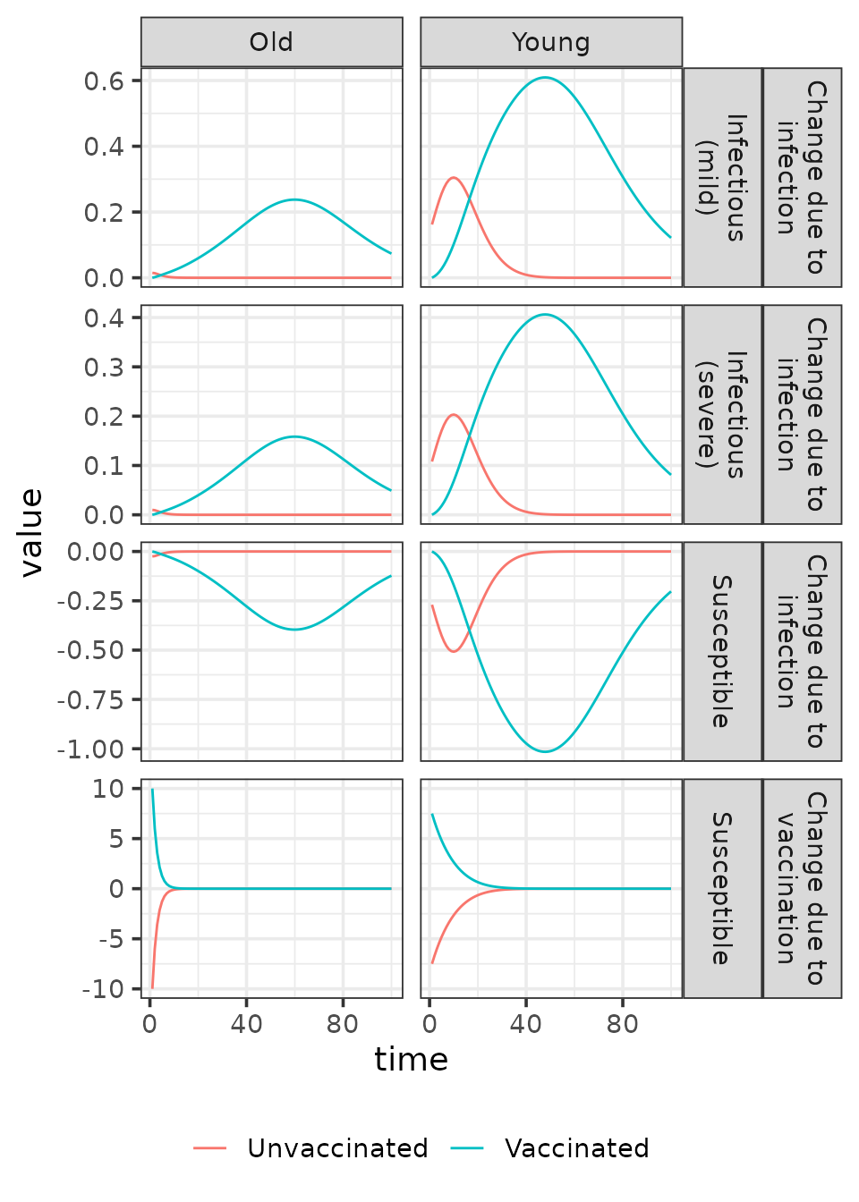
This plot reveals how susceptible individuals are allocated across symptom status compartments. By using color to represent vaccination status—instead of faceting into separate panels—it simultaneously highlights differences in rates of change across vaccination groups.

Limitations

One cannot use alternate state update methods with structured models, although this is on the roadmap.