Specifying Time-Varying Parameters

Baseline SIR Model

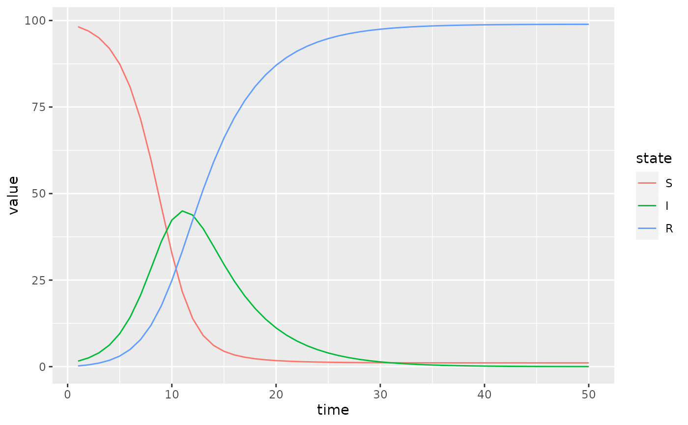
Here we modify an SIR model so that transmission rate is time-varying.

sir = Compartmental(system.file("starter_models", "sir", package = "macpan2"))
simulator = sir$simulators$tmb(time_steps = 50
  , state = c(S = 99, I = 1, R = 0)
  , flow = c(foi = 0, gamma = 0.2)
  , N = empty_matrix
  , beta = 0.8
)
(simulator$report(.phases = "during")
  %>% rename(state = row)
  %>% mutate(state = factor(state, sir$labels$state()))
  %>% ggplot() + geom_line(aes(time, value, colour = state))
)

Piecewise Time Variation

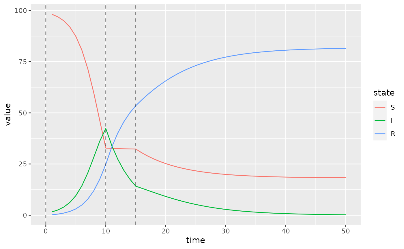
We now change the value of the transmission rate, beta, at the beginning of time-step 10 and 15. In the first step we add to the simulator a vector containing these change-points.

simulator$add$matrices(beta_changepoints = c(0, 10, 15))

Next we add the values to which beta changes at these time-steps.

simulator$add$matrices(beta_values = c(0.8, 0.01, 0.4))

We also need a variable to track the current value of beta. This beta_pointer starts at time-step equal to 0, and it will be incremented throughout the simulation.

simulator$add$matrices(beta_pointer = 0)

We increment beta_pointer using the time_group function that returns either beta_pointer or beta_pointer + 1 depending on whether or not the current time-step is at a change-point in beta_changepoints.

simulator$insert$expressions(
    beta_pointer ~ time_group(beta_pointer, beta_changepoints), 
    .phase = "during"
)

We update beta at every iteration of the simulation loop using this beta_pointer.

simulator$insert$expressions(
  beta ~ beta_values[beta_pointer],
  .phase = "during"
)

And that’s it. Now we plot the updated simulations using these change-points, which we highlight with vertical lines.

s = simulator$report(.phases = "during")
(s
  %>% rename(state = row)
  %>% mutate(state = factor(state, sir$labels$state()))
  %>% ggplot()
  + geom_line(aes(time, value, colour = state))
  + geom_vline(
    aes(xintercept = x), 
    linetype = "dashed", 
    alpha = 0.5, 
    data = data.frame(x = simulator$get$initial("beta_changepoints"))
  )
)

Calibrating Time Variation Parameters

First we simulate data to fit our model to, to see if we can recover the time-varying parameters.

set.seed(1L)
I_observed = rpois(
  50, 
  filter(s, matrix == "state", row == "I")$value
)
plot(I_observed)

Then we add a few matrices to the model for keeping tracking of information used in model fitting.

simulator$add$matrices(
  
  ## observed data
  I_obs = I_observed,
  
  ## simulated trajectory to compare with data
  I_sim = empty_matrix, 
  
  ## location of I in the state vector
  ## (the `-1L` bit is to get 0-based indices instead of 1-based)
  I_index = match("I", sir$labels$state()) - 1L, 
  
  ## matrix to contain the log likelihood values at 
  ## each time step
  log_lik = empty_matrix, 
  
  ## need to save the simulation history of each of these matrices
  .mats_to_save = c("I_sim", "log_lik")
)

Now we need some new expressions. The first expression pulls out the I state from the state vector.

simulator$insert$expressions(
  I_sim ~ state[I_index],
  .phase = "during"
)

The second expression computes a vector of Poisson log-likelihood values – one for each time step.

simulator$insert$expressions(
  log_lik ~ dpois(I_obs, clamp(rbind_time(I_sim))),
  .phase = "after"
)
simulator$replace$obj_fn(~ -sum(log_lik))

Next we declare the beta values as parameters to be optimized on the log scale.

simulator$add$transformations(Log("beta_values"))
simulator$replace$params(
  default = log(mean(simulator$get$initial("beta_values"))),
  mat = rep("log_beta_values", 3L),
  row = 0:2
)

Finally we fit the model back to the simulation data.

simulator$optimize$nlminb()
#> Constructing atomic D_lgamma
#> outer mgc:  736.1414 
#> Constructing atomic D_lgamma
#> outer mgc:  112.6655 
#> outer mgc:  71.38648 
#> outer mgc:  13.6616 
#> outer mgc:  12.58091 
#> outer mgc:  3.638083 
#> outer mgc:  1.399513 
#> outer mgc:  1.609453 
#> outer mgc:  1.140347 
#> outer mgc:  0.5870909 
#> outer mgc:  0.2527136 
#> outer mgc:  0.09938628 
#> outer mgc:  0.03753935 
#> outer mgc:  0.01394885 
#> outer mgc:  0.005150654 
#> outer mgc:  0.001897432 
#> outer mgc:  0.0006983805 
#> outer mgc:  0.0002569678 
#> outer mgc:  9.453969e-05 
#> outer mgc:  3.478009e-05 
#> outer mgc:  1.2795e-05 
#> outer mgc:  4.707033e-06 
#> outer mgc:  1.731623e-06 
#> outer mgc:  6.370286e-07 
#> outer mgc:  2.3435e-07 
#> outer mgc:  8.621247e-08 
#> outer mgc:  3.171579e-08
#> $par
#>      params      params      params 
#>  -0.1710158 -22.8268369  -0.8291142 
#> 
#> $objective
#> [1] 99.74231
#> 
#> $convergence
#> [1] 0
#> 
#> $iterations
#> [1] 26
#> 
#> $evaluations
#> function gradient 
#>       28       27 
#> 
#> $message
#> [1] "relative convergence (4)"

We can see that the optimizer converges (i.e. $convergence = 0) in 26 iterations.

On the log scale we see that the optimizer finds different values (current) than it started at (default).

simulator$current$params_frame()
#>   par_id             mat row col    default     current
#> 1      0 log_beta_values   0   0 -0.9079919  -0.1710158
#> 2      1 log_beta_values   1   0 -0.9079919 -22.8268369
#> 3      2 log_beta_values   2   0 -0.9079919  -0.8291142

More importantly the beta values on the untransformed scale recover to the values used in the simulations, although the second fitted beta value is much smaller than the true value.

data.frame(
  fitted = formatC(
    exp(simulator$current$params_frame()$current),
    format = "e", digits = 2
  ),
  true = simulator$get$initial("beta_values")
)
#>     fitted true
#> 1 8.43e-01 0.80
#> 2 1.22e-10 0.01
#> 3 4.36e-01 0.40

Smooth Time Variation (TODO)

Generalized Linear Models (TODO)

Generalized Linear Mixed Models (TODO)